When is it best to use a battery or a power supply for testing my battery powered device?

As I do quite a bit of work with mobile battery powered devices I regularly post articles here on our “Watt’s Up?” blog about aspects on testing and optimizing battery life for these devices. As a matter of fact my posting from two weeks ago is about the webcast I will be doing this Thursday, June 18^th: “Optimizing Battery Run and Charge Times of Today’s Mobile Wireless Devices”. That’s just two days away now!

With battery powered devices there are times it makes sense to use the device’s actual battery when performing testing and evaluation work to validate and gain insights on optimizing performance. In particular you will use the battery when performing a battery run-down test, to validate run-time. Providing you have a suitable test setup you can learn quite a few useful things beyond run-time that will give insights on how to better optimize your device’s performance and run-time. I go into a number of details about this in a previous posting of mine: “Zero-burden ammeter improves battery run-down and charge management testing of battery-powered devices”. If you are performing this kind of work you should find this posting useful.

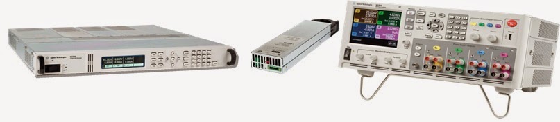
However, there are other times when it makes sense to use a power supply in place of the device’s battery, to power up the device for the purpose of performing additional types of testing and evaluation work for optimizing the device’s performance. One major factor for this is the power supply can be directly set to specific levels which remain fixed for the desired duration. It eliminates the variability and difficulties of trying to do likewise with a battery, if at all possible. In most all instances it is important that the power supply provides the correct characteristics to properly emulate the battery. This includes:

• Full two-quadrant operation for sourcing and sinking current and power
• Programmable series resistance to simulate the battery’s ESR

These characteristics are depicted in the V-I graph in figure 1.

Figure 1: Battery emulator power supply output characteristics

Note that quadrant 1 operation is emulating when the battery is providing power to the device while quadrant 2 is emulating when the battery is being charge by the device.

A colleague here very recently had an article published that goes into a number of excellent reasons why and when it is advantageous to use a power supply in place of trying to use the actual battery, “Simulating a Battery with a Power Supply Reaps Benefits”. I believe you will find this to also be a useful reference.

Simulating battery contact bounce, part 1

One test commonly done during design validation of handheld battery powered devices is to evaluate their ability to withstand a short loss of battery power due to being bumped and the contacts momentarily bouncing open, and either remain operating or have sufficient time to handle a shutdown gracefully. The duration of a contact bounce can typically range anywhere from under a millisecond to up to 100 milliseconds long.

To simulate battery contact bouncing one may consider programming a voltage drop out on a reasonably fast power supply with arbitrary waveform capabilities, like several of the N675xA, N676xA, or N678xA series modules used in the N6700 series Modular DC Power System or N6705B DC Power Analyzer mainframe, shown in Figure 1. It is a simple matter to program a voltage dropout of specified duration. As an example a voltage dropout was programmed in Figure 2 on an N6781A SMU module using the companion 14585A software.

 Figure 1: N6700 series and N6705B mainframes and modules

Figure 2: Programming a voltage drop out using the N6705B and N6781A SMU module

While a voltage dropout is fine for many applications, like automotive, in many situations it does not work well for simulating battery contact bounce. The reason for this is there is one key difference to note about a voltage dropout versus a battery contact bounce. During a voltage dropout the source impedance remains low. During a battery contact bounce the source impedance is an open circuit. However, a DC source having the ability to generate a fast voltage dropout is a result of it being able to pull its output voltage down quickly. This is due to its ability to sink current as well as source current. The problem with this is, for many battery powered devices, this effectively short-circuits the battery input terminals, more than likely causing the device to instantly shut down by discharging any carry-over storage and/or disrupting the battery power management system. As one example consider a mobile device having 50 microfarads of input capacitance and draws 4 milliamps of standby current. This capacitance would provide more than adequate carryover for a 20 millisecond battery contact bounce. However, if a voltage dropout is used to simulate battery contact bounce, it immediately discharges the mobile device’s input capacitance and pulls the battery input voltage down to zero, as shown by the red voltage trace in Figure 3. The yellow trace is the corresponding current drain. Note the large peaks of current drawn that discharge and recharge the DUT’s input capacitor.

 Figure 3: Voltage dropout applied to DUT immediately pulls voltage down to zero

One effective solution for preventing the DC source from shorting out the battery input is to add a DC blocking diode in series with the battery input, so that current cannot flow back out, creating high impedance during the dropout. This is illustrated in Figure 4.

Figure 4: Blocking diode added between SMU and DUT

One thing to note here is the diode’s forward voltage drop needs to be compensated for. Usually the best way to do this just program the DC source with the additional voltage needed to offset the diode’s voltage drop. The result of this is shown in Figure 5. As shown by the red trace the voltage holds up relatively well during the contact bounce period. Because the N6781A SMU has an auxiliary voltage measurement input it is able to directly measure the voltage at the DUT, on the other side of the blocking diode, instead of the output voltage of the N6781A. As seen by the yellow current trace there is no longer a large peak of current discharging the capacitor due to the action of the blocking diode.

 Figure 5: Blocking diode prevents voltage dropout from discharging DUT 

Now you should have a much better appreciation of the differences between creating a voltage dropout and simulating battery contact bounce! And as can be seen a blocking diode is a rather effective means of simulating battery contact bounce using a voltage dropout. Stay tuned for my second part on additional ways of simulating battery contact bounce on an upcoming posting.

.

What does it mean when my Agilent power supply displays “Osc”?

When using certain higher performance power supplies from Agilent, like the N678xA series source-measure modules, you may discover that the output has shut down and an annunciator displaying “Osc” shows up on the front panel meter display, like that shown in Figure 1 for the N6705B DC Power Analyzer mainframe. 

Figure 1: DC Power Analyzer front panel meter displaying “Osc” on channel 1 output

As you would likely guess, Osc stands for oscillation and this means the output has been shut down for an oscillation fault detection. In this particular instance an N6781A high performance source measure module was installed in channel 1 of the N6705B DC Power Analyzer mainframe.

The N678xA series source measure modules have very high bandwidth so that they can provide faster transient response and output slew rates. However, when the bandwidth of the power supply is increased, its output stability becomes more dependent on the output wiring and DUT impedances. To provide this greater bandwidth and at the same time accommodate a wider range of DUTs on the N678xA modules, there are multiple compensation ranges to select from, based on the DUT’s input capacitance, as shown in the advanced source settings screen in Figure 2.

Figure 2: DC Power Analyzer front panel displaying advanced source settings for the N678xA

Note that “Low” compensation range supports the full range of DUT loading capacitance but this is the default range. While it provides the most robust stability, it does not have the faster response and better performance of the “High” compensation ranges.

As long as the wiring to the DUT is correctly configured and an appropriate compensation range is selected the output should be stable and not trip the oscillation protection system. In the event of conditions leading to an unstable condition, any detection of output oscillations starting up quickly shut down the output in the manner I captured in Figure 3. I did this by creating an instability by removing the load capacitance.

Figure 3: Oscillation protection being tripped as captured in companion 14585A software

In rare circumstances, such as with some DUTs drawing extremely high amplitude, high frequency load currents, which may lead to false tripping, the oscillation protection can be turned off, as shown in Figure 4.

Figure 4: N678xA oscillation protection disable in N6705B DC Power Analyzer advance protection screen

Oscillation protection is a useful mechanism that can protect your DUT and your power supply from an excessively high AC voltage and current due to unstable operating conditions. Now you know what it means next time you see “Osc” displayed on the front panel of you Agilent power supply and what you need to do to rectify it!

.

European Space Power Conference (ESPC) for 2014

This week’s blog posting is going in a bit of a different direction, as I likewise did last month, to attend and participate in the 2014 European Space Power Conference (ESPC) for 2014. While this was the tenth ESPC, which I understand takes place every couple of years; this was the first time I had opportunity to attend. One thing for certain; this was all about DC power, which is directly aligned with the things I am always involved in. In this particular instance it was all about DC power for satellites and space-bound crafts and probes.

I initially found it just a bit curious that a number of the keynote speeches also focused a fair amount on terrestrial solar power as well, but I supposed I should not be at all surprised. There has been a large amount of innovation and a variety of things that benefit our daily lives that came out of our own space program, fueled by our involvement in the “space race” and still continuing on to this day. (Can you name a few by chance?). This is a natural progression for a vast number of technological advances we enjoy.

At ESPC there were numerous papers presented on solar cells and arrays, batteries and energy storage, nuclear power sources, power conversion and DC/DC converters, super-capacitors, and a variety of other topics related to power. Just a couple of my learnings and observations include:

·         There was a very high level of collaboration of sharing findings and answering questions among peers attending the event

·         While batteries generally have very limited lives, from findings presented, it was interesting to see how well they have performed over extended periods in space, lasting last well in excess of their planned life expectancies. It is a reflection of a combination of several things including careful control and workmanship, understanding life-shortening and failure mechanisms, how to take properly treat them over time, what should be expected, as well as other factors contributing to their longevity. I expect this kind of work will ultimately find its way to being applied to using lithium ion batteries in automotive as well.

·         A lot of innovation likewise continues with solar cell development with higher conversion efficiencies coming from multi-junction devices. Maybe we’ll see this become commonplace for terrestrial applications before long!

·         A number of research papers were presented from participants from universities as well. In all, the quality of work was excellent.

I was there with another colleague, Carlo Canziani. Together we represented some of our DC power solutions there, including our N7905A DC Power Analyzer, N7900 series Advanced Power System (APS), and E4360A series Solar Array Simulator (SAS) mainframe and modules. These are the kinds of advanced power stimulus and measurement test instruments vital for conducting testing on satellite and spacecraft power components and systems.

In all it was a refreshing change of pace to be at an event where power is the primary focus, and if this happens to be an area of interest to you as well, you can find out more about ESPC from their site by clicking on the following link: (ESPC2014). Maybe you will find it worthwhile to attend or even present results of some of your work at the next one as well!

Upcoming software release unleashes the N7900 APS’s potential without any programming

Our N7900A Advanced Power System (APS) is well named, being the most advanced power product we’ve introduced to date. In many ways it is based on our N6700 series modular DC power system and N6705B DC power analyzer, incorporating their capabilities, including:

• High precision programming and measurement
• Seamless measurement ranging
• High speed measurement digitization of voltage, current, and power
• Long term data logging of voltage, current, and power
• Output ARB and List capabilities
• And quite a bit more

In addition the N7900A APS brings quite a few new and unique capabilities as well, including:

• Much greater output power
• Logic-configurable expression signal routing for advanced custom triggering and control
• Optional external dissipater unit for full two quadrant operation
• Optional black box recorder for post-test diagnostics when needed
• And quite a bit more

To take advantage of these advance capabilities does require a bit of programming, which is to generally be expected for an automated test environment, but in low volume design validation and R&D this can slow down the desired quick time-to-result. The N6705B DC Power Analyzer, in Figure 1, has a full-featured front panel menu and graphical display that lets design validation and R&D users quickly configure and run complex power-related tests on their devices. In comparison, the N6700 series, pictured in Figure 2, does not have all the front panel capabilities of the N6705B and can be looked on as the ATE version of this product platform, requiring programming to take advantage of its advanced capabilities. The N6705B shares all the same DC power modules that the N6700 series uses.

Figure 1: The N6705B DC Power Analyzer, primarily for bench use

Figure 2: The N6700 series Modular DC Power System, primarily for ATE

The N7900A APS is very similar in form and function to the N6700 series, not having all the advanced front panel capabilities that the N6705B has for bench-friendly use of its advanced features. I am really pleased to be able to share with you that this is now changing! While we are not creating a bench version of the N7900 APS, we are upgrading our 14585A Control and Analysis software, which emulates the front panel of an N6705B and more, to work with the N7900 APS as well. The 14585A will soon let you quickly and easily create and configure complex power-related tests based on using the N7900 APS.  I am fortunate enough to be working with a beta version of the software. Some examples of things I was able to do in just a few minutes were to capture the inrush current of an automotive headlight, shown in Figure 3, and superimpose an AC sine wave disturbance on top of the DC output, shown in Figure 4.

Figure 3: Auto headlamp inrush current captured with 14585A software and N7951A APS

Figure 4: Sine wave voltage disturbance on top of DC generated by 14585A software and N7951A APS

The updated release of the 14585A Control and Analysis software is just a few weeks away. More about the 14585A software can be found by clicking on the following link <14585A>. With the 14585A being a great way to implement ideas and tests quickly, using the N7900 APS, look for me and others coming up with some interesting applications in future posts here on “Watt’s Up?”!

How to test the efficiency of DC to DC converters, part 2 of 2

In part 1 of my posting on testing the efficiency of DC to DC converters (click here to review) I went over the test set up, the requirements for load sweep synchronized to the measurements, and details of the choice of the type and set up of the current load sweep itself. In this second part I will be describing details of the measurement set up, setting up the efficiency calculation, and results of the testing. This is based on using the N6705B DC Power Analyzer, N6782A SMUs, and 14585A software as a platform but a number of ideas can be applicable regardless of the platform.

Figure 1: Synchronized measurement and efficiency calculation set up

The synchronized measurement and efficiency calculation set up, and display of results are shown in Figure 1, taking note of the following details corresponding to the numbers in Figure 1:

1. In the 14585A the data logging mode was selected to make and display the measurements. The oscilloscope mode could have just as easily been used but with a 10 second sweep the extra speed of sampling with the oscilloscope mode was not an advantage. A second thing about using the data logging mode is you can set the integration time period for each acquisition point. This can be used to advantage in averaging out noise and disturbances as needed for a smoother and more representative result. In this case an integration period of 50 milliseconds was used.
2. To synchronize the measurements the data log measurement was set to trigger off the start of the load current sweep.
3. Voltage, current, and power for both the input and output SMUs were selected to be measured and displayed. The input and output power are needed for the efficiency calculation.
4. The measurements were set to seamless ranging. In this way the appropriate measurement range for at any given point was used as the loading swept from zero to full load.
5. A formula trace was created to calculate and display the efficiency in %. Note that the negative of the ratio of output power to input power was used. This is because the SMU acting as a load is sinking current and so both its current and power readings are negative.

With all of this completed really all that is left to do is first start the data logging measurement with the start button. It will be “armed” and waiting from a trigger signal from the current load sweep ARB that had been set up. All that is now left to do is press the ARB start button. Figure 2 is a display of all the results after the sweep is completed.

Figure 2: DC to DC Converter efficiency test results

All the input and output voltage, current, and power measurements, and efficiency calculation (in pink) are display, but it can be uncluttered a bit by turning off the voltages and currents traces being displayed and just leave the power and efficiency traces displayed. This happened to be special DC to DC converter designed to give exceptionally high efficiency even down to near zero load, which can be seen from the graph. It’s interesting to note peak efficiency occurred at around 60% of full load and then ohmic losses start becoming more significant.

And that basically sums it all up for performing an efficiency test on a DC to DC converter!

Power analysis of automobile self-charging emergency tool

I was recently given a “Swiss+Tech BodyGard Survivor 8-in-1 Automobile Self-Charging Emergency Tool”. How’s that for a compact name? This device does have many features, so I imagine the company had some difficulty devising a name for it. It is meant to be carried in your car and kept close enough to the driver to be used in an emergency. It contains a glass breaker, a seatbelt cutter, a flashlight, an emergency flasher and siren, an AM/FM radio, and rechargeable NiCad batteries that charge by using the self-charging hand crank. See Figure 1.

Since this device contains rechargeable batteries and Agilent makes instrumentation that can do battery drain analysis, I figured I would test the device using our equipment. I used an Agilent N6705B DC Power Analyzer loaded with an N6781A 2-Quadrant Source/Measure Unit (SMU) for Battery Drain Analysis. See Figure 2.

The product’s instruction sheet includes information about the batteries (700 mAH) and the expected battery run time when using the various features. With fully charged batteries, the expected battery run time for each of the features listed below is:

• Flashlight: 12 to 16 hours
• Flasher: 10 to 12 hours
• Radio (low volume): 35 to 40 hours
• Flasher/siren: 6 to 9 hours

Given the battery amp-hour rating (700 mAH) and the expected run time in hours, we can calculate the approximate expected average current draw for each of the various features:

• Flashlight: 700 mAH / 14 hours = 50 mA
• Flasher: 700 mAH / 11 hours = 63.6 mA
• Radio: 700 mAH / 37.5 hours = 18.7 mA
• Flasher/siren: 700 mAH / 7.5 hours = 93 mA

Using the N6781A SMU and the built-in front panel features of the N6705B DC Power Analyzer, I was able to analyzer the current drawn from the batteries when using each of the features. Each feature was used by itself with the other features turned off.

The flashlight draws a steady-state current that I read right from the front panel meter as shown in Figure 3: 50 mA. This agrees perfectly with the expected current draw I calculated. For this measurement and all subsequent current measurements, I connected the N6781A in series with the batteries and set it to Current Measure mode where it acts likes a zero-burden shunt. The measured current is negative in my setup because positive current is current flowing into the battery and with the flashlight on, current is flowing out of the battery.

For the flasher, since the current is not constant, I used the N6705B/N6781A built-in data logger feature and captured 30 seconds of data while the device was flashing. I then used the markers to measure the average current. Since the flasher flashes for a very short period of time (low duty cycle), I expected the average current to be low. When using the flasher, the expected battery run time seemed unusually short to me. At 10 to 12 hours, it is shorter than the flashlight or radio run time, which seems odd. In reality, as shown in Figure 4, the flasher drew very little current (5.6 mA), so it appears that the instruction sheet run time for the flasher is too low. With the device flashing, the battery will last much longer than indicated. In fact, the expected battery run time, when flashing, is about 700 mAH / 5.6 mA = 125 hours, 10 times longer than the time shown on the instruction sheet!

With the radio on, tuned to a station, and set to a low but audible volume, I once again used the data logger to capture the current. The markers show an average current of about 10 mA, which is less than the calculated value of 18.7 mA, but within reason. See Figure 5.

Using the flasher and siren, the data logger shows a current draw of 93 mA, in exact agreement with the expected current draw calculated from the numbers on the instruction sheet. See Figure 6.

The last current analysis I did was to capture 30 seconds of data logging when turning the self-charging crank to recharge the batteries. I purposely varied my cranking rate to see what would happen. Figure 7 shows an average of about 350 mA when turning the crank at what I considered to be a typical rate (highest average numbers on the captured data log). To fully charge 700 mAH batteries, it would take about 2 hours at that rate, which is in agreement with the instruction sheet (it says 2 to 3 hours). I don’t know about you, but I don’t want to turn that crank for 2 hours straight! Let’s hope I never have to use the tool for real, but I’m glad I have it just in case!

How do I measure inrush current with an Agilent DC Power Supply?

Hello everybody! I want to build on my blog post from last month.  This month, we are going to discuss how to measure inrush current using the DC Power Analyzer’s scope function as well as the digitizer feature that is available on some of our system power supplies.

Measuring inrush current is a task that many customers that use DC Power Supplies want to accomplish.  When you are doing this test on the bench, the N6705B DC Power Analyzer (DCPA) is your best bet.  The DCPA has the scope feature which makes this a breeze.  One of the great things about Agilent power supplies is that they can measure current directly, without the need for a current probe. Some of our supplies have very high current measurement accuracy as well so you can get an accurate representation of your current.

In the below screenshot, I just had a capacitor connected to the output of the supply.  I set a voltage arbitrary waveform that went from 0 V to 20 V with the voltage slew set for the maximum.  I set the scope to trigger on the Arb run/stop key so that when I hit the key, both the arbitrary waveform and the scope triggered.  After I acquired the waveform, I used the markers to get the maximum current.  That number is our inrush current.   

As I said earlier, DCPA is geared towards bench use.   The graphical scope makes this task pretty easy.  Many of our system supplies (as well as the DCPA) have a digitizer feature that you can access using the SCPI programming interface.  The digitizer will sample the output using settings that you provide it.  These settings are: the number of points, the time interval between points, and the number of pretrigger points that you acquire.  In the N678xA SMU modules, the time interval is as low as 5.12 us and the number of points is as high as 512kpoints.  Here is a list of commands to set up the digitizer (written for the N67xx supplies) as well as some comments.

Set the digitizer to measure current:

 SENS:FUNC:CURR ON,(@1)

Set the number of pretrigger points, a negative value represents points taken before the trigger:

SENS:SWE:OFFS:POIN -100,(@1)

Set the total number of points to acquire:

SENS:SWE:POIN 5000,(@1)

Set the time interval between points:

SENS:SWE:TINT 0.000020,(@1)

Set the measurement trigger source to bus:

TRIG:ACQ:SOUR BUS,(@1)

 Initiate the measurement trigger system

INIT:ACQ (@1)

Send a trigger:

*TRG

Using this code, once the trigger is sent, the measurement system will acquire 5000 points at a time interval of 20 us while taking 100 pretrigger points. 

After the measurement occurs, you read the current back using:

FETC:ARR:CURR? (@1)

Once you have the array of current measurements, you can do any normal calculation that you can do on any array.  To measure inrush, you want to find the maximum current in the array.  This peak will be your inrush current.  I wrote a program that followed the exact same steps that I used on the scope above (setting up a step that went from 0 to 20 V and synchronizing triggers) and measured a maximum of 1.07748 A.  As you can see, I got a similar result from the two different approaches.

That is all that I have this month.  I hope that it is useful information.  If you have any questions at all please feel free to ask them in our comments.