Showing posts with label current level. Show all posts

Tuesday, November 18, 2014

Why does the response time of OCP vary on the power supply I am using and what can I do about it? Part 1

In a previous posting of mine “Providing effective protection of your DUT against over voltage damage during test”(click here to review), an important consideration for effective protection was to factor in the response time of the over voltage protect (OVP) system. Due to the nature of over voltage damage, the OVP must be reasonably fast. The response time can typically be just a few tens of microseconds for a reasonably fast OVP system on a higher performance system power supply to hundreds of microseconds on a more basic performance system power supply. This response time usually does not vary greatly with the amount of over voltage being experienced.

Just as with voltage, system power supplies usually incorporate over current protect (OCP) systems as well. But unlike over voltage damage, which is almost instantaneous once that threshold is reached, over current takes more time to cause damage. It also varies in some proportion to the current level; lower currents taking a lot longer to cause damage. The I2t rating of an electrical fuse is one example that illustrates this effect.

Correspondingly, like OVP, power supply OCP systems also have a response time. And also like OVP, the test engineer needs to take this response time into consideration for effective protection of the DUT.  However, unlike OVP, the response time of an OCP system is quite a bit different. The response time of an OCP system is illustrated in Figure 1.


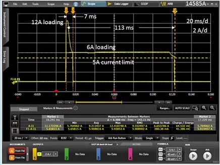
Figure 1: Example OCP system response time vs. overdrive level

Here in Figure 1 the response time of the OCP system of a Keysight N7951A 20V, 50A power supply was characterized using the companion 14585A software. It compares response times of 6A and 12A loading when the current limit is set to 5A. Including the programmed OCP delay time of 5 milliseconds it was found that the actual total response time was 7 milliseconds for 12A loading and 113 milliseconds for 6A loading.

This is quite different than the response time of an OVP system. Even if the OCP delay time was set to zero, the response is still on the order of milliseconds instead of microseconds for the OVP system. And when the amount of overdrive is small, as is the case for the 6A loading, providing just 1A of overdrive, the total response time is much greater. Why is that?

Unlike the OVP system, which operates totally independent of the voltage limit control system, the OCP system is triggered off the current limit control system. Thus the total response time includes the response time of the current limit as well. The behavior of a current limit is quite different than a simple “go/no go” threshold detector as well. A limit system, or circuit, needs to regulate the power supply’s output at a certain level, making it a feedback control system. Because of this stability of this system is important, both with crossing over from constant voltage operation as well as maintaining a stable output current after crossing over. This leads to the slower and overdrive dependent response characteristics that are typical of current limit systems.

So what can be done about the slower response of an OCP system? Well, early on in this posting I talked about the nature of over current damage. Generally over current damage is much slower by nature and the over drive dependent response time is in keeping with time dependent nature of over current damage. The important thing is understand what the OCP response characteristic is like and what amount of over current your DUT is able to sustain, and you should be able to make effective use of the over current protection capabilities of your system power supply.

If however you are still looking how you might further improve on OCP response speed, look for my follow up to this in my next posting!

Monday, April 8, 2013

Why would a DC power supply have RMS current readback?


During a conversation with a colleague at work one day the topic of having RMS current readback on DC power supplies came up. It is a measurement capability we have on a number of our system DC power supplies. He posed the question: Why the reason for having such a capability? I actually had not been involved with the original investigations identifying what reasons this was added so I instead had to rely on my intuition. That’s not always a good thing but it did help me out this time at least!

He had argued that since you are feeding a fixed DC voltage into the device you are powering, the power consumption is going to be a product of the DC (average) voltage and DC (average) current, regardless of whether the current is purely DC, or if it is dynamic, having a substantial amount of AC content. This is true, as I have illustrated in figure 1, comparing purely DC and pulsed currents being drawn by a load. For purely DC current the DC and RMS values are the same. In comparison, for a pulsed current the RMS value is greater the DC value. Regardless, the RMS current value does not factor into the overall power consumption of the DUT here. The power consumption is still the product of the DC voltage and current.


Figure 1: Comparing power consumption of a DC powered DUT drawing constant and pulsed currents

So why provide an RMS current measurement? Well there can be times when this can prove useful, even when the DUT is powered by a fixed DC voltage. Consider the scenario depicted in Figure 2.


Figure 2: Properly sizing a protection fuse on a DC powered device

Many products incorporate fuses to protect from over-current and subsequent damage, usually brought on due to misuse or component failure. Fuses are rated by their RMS current handling, not the DC current. In the case of the pulsed loading the RMS current is twice the DC current and the resulting power in the fuse is four times that for a constant current.  If the fuse was selected based on the DC current value it would most certainly fail well below the required operating level!

My colleague conceded that this fuse example was a legitimate case where RMS current measurement would indeed be useful. Maybe it was not a frivolous capability after all. No doubt sizing fuses is just one of many reasons why RMS measurement on DC products can be useful!

Monday, December 10, 2012

More on power supply current source-to-sink crossover characteristics


On my earlier posting “Power supply current source-to-sink crossover characteristics” I showed what the effects on the output voltage of a unipolar two-quadrant-power supply were, resulting from the output current on the power supply transitioning between sourcing and sinking. In that example scenario, the power supply was maintaining a constant output voltage and the transitioning between sourcing and sinking current was dictated by the external device connected to and being powered by the power supply. This is perhaps the most common scenario one will encounter that will drive the power supply between sourcing current and sinking current.

Other scenarios do exist that will drive a unipolar two-quadrant power supply to transition between sourcing and sinking output current. One scenario is nearly identical to the earlier posting. However, instead of the device transitioning its voltage between being less and greater than the power supply powering it, the power supply instead transitions its voltage between being less and greater than the active device being normally powered.  A set up for evaluating this scenario on an Agilent N6781A two-quadrant DC source is depicted in Figure 1.


Figure 1: Evaluating current source-to-sink crossover on an N6781A operating in constant voltage

In this scenario having the DC source operating as a voltage source and transitioning between 1.5 and 4.5 volts causes the current to transition between -0.75 and +0.75A.  The voltage and current waveforms captured on an oscilloscope are shown in Figure 2.


Figure 2: Voltage and current waveforms for the set up in Figure 1

The waveforms in Figure 2 are as what should be expected. The actual transition points are where the current waveform passes through zero on the rising and falling edge. An expanded view to the current source-to-sink transition is shown in Figure 3.


Figure 3: Expanded voltage and current waveforms for the set up in Figure 1

As can be seen the voltage ramp transitions smoothly at the threshold point, or zero crossing point, of the current waveform. The reason being is that the DC is maintaining its operation as a voltage source. Its voltage feedback loop is always in control.


Yet one more scenario that will drive a unipolar two-quadrant source to transition between sourcing and sinking current is operate it as a current source and program is current setting between positive and negative values. In this case the device under test that was used is a voltage source.  One real-world example is cycling a rechargeable battery by alternately applying charging and discharging currents to it. The set up for evaluating this scenario, again using an N6781A two-quadrant DC source is depicted in Figure 4.


Figure 4: Evaluating current source-to-sink crossover on an N6781A operating in constant current

For Figure 4 the N6781A was set to operate in constant current and programmed to alternately transition between -0.75A and +0.75A current settings. The resulting voltage and current waveforms are shown in Figure 5.


Figure 5: Voltage and current waveforms for the set up in Figure 4

The waveforms in Figure 5 are as what should be expected. The actual transition points are where the current waveform passes through zero on the rising and falling edge. An expanded view to the current source-to-sink transition is shown in Figure 6.


Figure 6: Expanded voltage and current waveforms for the set up in Figure 4

As the N6781A is operating in current priority the interest is in how well it controls its current while transitioning through the zero-crossing point. As observed in Figure 6 it transitions smoothly through the zero-crossing point. The voltage performance is determined by the DUT, not the N6781A, as the N6781A is operating in constant current.

So what was found here is, for a unipolar two-quadrant DC source, transitioning between sourcing and sinking current should generally be virtually seamless as, under normal circumstances, should remain in either constant voltage or constant current during the entire transition.

Tuesday, August 7, 2012

How Does an Electronic Load Regulate It’s Input Voltage, Current, and Resistance?


In a sense electronic loads are the antithesis of power supplies, i.e. they sink or absorb power while power supplies source power. In another sense they are very similar in the way they regulate constant voltage (CV) or constant current (CC). When used to load a DUT, which inevitably is some form of power source, conventional practice is to use CC loading for devices that are by nature voltage sources and conversely use CV loading for devices that are by nature current sources. However most all electronic loads also feature constant resistance (CR) operation as well. Many real-world loads are resistive by nature and hence it is often useful to test power sources meant to drive such devices with an electronic load operating in CR mode.

To understand how CC and CV modes work in an electronic load it is useful to first review a previous posting I wrote here, entitled “How Does a Power Supply Regulate It’s Output Voltage and Current?”. Again, the CC and CV modes are very similar in operation for both a power supply and an electronic load. An electronic load CC mode operation is depicted in Figure 1.


Figure 1: Electronic load circuit, constant current (CC) operation

The load, operating in CC mode, is loading the output of an external voltage source. The current amplifier is regulating the electronic load’s input current by comparing the voltage on the current shunt against a reference voltage, which in turn is regulating how hard to turn on the load FET. The corresponding I-V diagram for this CC mode operation is shown in Figure 2. The operating point is where the output voltage characteristic of the DUT voltage source characteristic intersects the input constant current load line of the electronic load.


Figure 2: Electronic load I-V diagram, constant current (CC) operation

CV mode is very similar to CC mode operation, as depicted in Figure 3.  However, instead of monitoring the input current with a shunt voltage, a voltage control amplifier compares the load’s input voltage, usually through a voltage divider, against a reference voltage. When the input voltage signal reaches the reference voltage value the voltage amplifier turns the load FET on as much as needed to clamp the voltage to the set level.


Figure 3: Electronic load circuit, constant voltage (CV) operation

A battery being charged is a real-world example of a CV load, charged typically by a constant current source. The corresponding I-V diagram for CV mode operation is depicted in figure 4.


Figure 4: Electronic load I-V diagram, constant voltage (CV) operation

But how does an electronic load’s CR mode work? This requires yet another configuration, as depicted in figure 5. While CC and CV modes compare current and voltage against a reference value, in CR mode the control amplifier compares the input voltage against the input current so that one is the ratio of the other, now regulating the input at a constant resistance value.  With current sensing at 1 V/A and voltage sensing at 0.2 V/V, the electronic load’s resulting  input resistance value is 5 ohms for its CR mode operation in Figure 5.


Figure 5: Electronic load circuit, constant resistance (CR) operation

An electronic load’s CR mode is well suited for loading a power source that is either a voltage or current source by nature. The corresponding I-V diagram for this CR mode for loading a voltage source is shown in Figure 6. Here the operating point is where the output voltage characteristic of the DUT voltage source intersects the input constant resistance characteristic of the load.


Figure 6: Electronic load I-V diagram, constant resistance (CR) operation

As we have seen here an electronic load is very similar in operation to a power supply in the way it regulates to maintain constant voltage or constant current at its input.  However many real-world loads exhibit other characteristics, with resistive being most prevalent. As a result most all electronic loads are alternately able to regulate their input to maintain a constant resistance value, in addition to constant voltage and constant current.

Tuesday, July 17, 2012

How Does a Power Supply regulate It’s Output Voltage and Current?


We have talked about Constant Voltage (CV) and Constant Current (CC) power supply operation in many various ways and applications here on the “Watt’s Up?” blog in the past. Indeed, CV and CC are fundamental operating modes of most all power supplies. But what exactly takes place inside the power supply that endows it with the ability to regulate either its output voltage or current, depending on the load? If you ever wondered about this, wonder no longer!

Most all power supplies regulate either their output voltage or output current at a constant level, depending on the load resistance relative to the power supply’s output voltage and current settings. This can be summarized as follows:

·         If R load > (V out / I out) then power supply is in CV mode
·         If R load < (V out / I out) then power supply is in CC mode

To accomplish this most all power supplies have separate voltage and current feedback control loops to limit either the output voltage or current, depending on the load. To illustrate this Figure 1 shows a circuit diagram of a basic 5 volt, 1 amp output series regulated power supply operating in CV mode.


Figure 1: Basic DC Power Supply Circuit, Constant Voltage (CV) Operation

The CV and CC control loops/amplifiers each have a reference input value. In this case the reference values are both 1 volt. In order to regulate output voltage the CV error amplifier compares its 1 volt reference against a resistor divider that divides the output voltage down by a factor of 5, limiting the output voltage to 5 volts. Likewise the CC error amplifier compares its 1 volt reference against a 1 ohm current shunt resistor located in the output current path, limiting the output current to 1 amp. For Figure 1 the load resistance is 10 ohms. Because this load resistance is greater than (V out / I out) = 5 ohms, the power supply is operating in CV mode. The CV error amplifier takes control of the series pass transistor by drawing away excess base current from the series pass transistor, though the diode “OR” network. The CV amplifier is operating in closed loop, maintaining its error voltage at zero volts. In comparison, because the actual output current is only 0.5 amps the CC amplifier tries to turn the current on harder but cannot because the CV amplifier has control of the output. The CC amplifier is operating open loop. Its output goes up to its positive limit while it has -0.5 volts of error voltage. The output I-V diagram for this Constant Voltage operation is shown in Figure 2.


Figure 2: Power Supply I-V Diagram, CV Operation

Now say we increase the load by lowering the output load resistance from 10 ohms down to 3 ohms. Figure 3 shows the circuit diagram of our basic 5 volt, 1 amp output series regulated power supply revised for operating in CC mode with a 3 ohm load resistor.


Figure 3: Basic DC Power Supply Circuit, Constant Current (CC) Operation

Because the load resistor is lower than (V out / I out) = 5 ohms, the power supply switches to CC mode. The CC error amplifier takes control when the voltage drop on the current shunt resistor increases to match the 1 volt reference value, corresponding to 1 amp output, drawing excess base current from the series pass transistor though the diode “OR” network. The CC amplifier is now operating closed loop, regulating the output current to maintain its input error voltage at zero. In comparison, because the actual output voltage is now only 3 volts the CV amplifier tries to increase the output voltage but cannot because the CC amplifier has control of the output. The CV amplifier is operating open loop. Its output now goes up to its positive limit while it has -0.4 volts of error voltage. The output I-V diagram for this Constant Current operation is shown in Figure 4.


Figure 4: Power Supply I-V Diagram, CC Operation

As we have seen most all power supplies have separate current and voltage control loops to regulate their outputs in either a Constant Voltage (CV) or in a Constant Current (CC) mode. One or the other takes control, depending on that the load resistance is in relation to what the power supply’s output voltage and current settings are. In this way both the load and power supply are protected by limiting the voltage and current that is delivered by the power supply to the load. By understanding this theory behind a power supply’s CV and CC operation it is also easier to understand the underlying reason for why various power supply characteristics are the way they are, as well as see how other power supply capabilities can be created by building on top of this foundation. Stay tuned!

Tuesday, May 8, 2012

Establishing Measurement Integration Time for Leakage Currents

The proliferation of mobile wireless devices drives a corresponding demand for components going into these devices. A key attribute of these components is the need to have low levels of leakage current during off and standby mode operation, to extend the battery run-time of the host device. I brought up the importance of making accurate leakage currents quickly in an earlier posting “Pay Attention to the Impact of the Bypass Capacitor on Leakage Current Value and Test Time”(click here to review). Another key aspect about making accurate leakage currents quickly is establishing the proper minimum required measurement integration time. I will go into factors that govern establishing this time here.

Assuming the leakage current being drawn by the DUT, as well as any bypass capacitors on the fixture, have fully stabilized, the key thing with selecting the correct measurement integration time is getting an acceptable level of measurement repeatability. Some experimentation is useful in determining the minimum required amount of time. The primary problem with leakage current measurement is one of AC noise sources present in the test set up. With DC leakage current being just a few micro amps or less these noises are significant. Higher level currents can be usually measured much more quickly as the AC noises are relatively negligible in comparison. There are a variety of potential noise sources, including radiated and conducted from external sources, including the AC line, and internal noise sources, such as the AC ripple voltage from the DC source’s output. This is illustrated in Figure 1 below. Noise currents directly add to the DC leakage current while noise voltages become corresponding noise currents related by the DUT and test fixture load impedance.


Figure 1: Some noise sources affecting DUT current measurement time

Using a longer measurement time integrates out the peak-to-peak random deviations in the DC leakage current to provide a consistently more repeatable DC measurement result, but at the expense of increasing overall device test time. Measurement repeatability should be based on a statistical confidence level, which I will do into more detail further on. Using a measurement integration time of exactly one power line cycle (1 PLC) of 20 milliseconds (for 50 Hz) or 16.7 milliseconds (for 60 Hz) cancels out AC line frequency noises. Many times a default time of 100 milliseconds is used as it is an integer multiple of both 20 and 16.7 milliseconds. This is fine if overall DUT test time is relatively long but generally not acceptable when total test time is just a couple of seconds, as is the case with most components. As a minimum, setting the measurement integration time to 1 PLC is usually the prudent thing to do when short overall DUT test time is paramount.

Reducing leakage current test time below 1 PLC means reducing any AC line frequency noises to a sufficiently low level such that they are relatively negligible compared to higher frequency noises, like possibly the DC source’s wideband output ripple noise voltage and current. Proper grounding, shielding, and cancellation techniques can greatly reduce noise pickup. Paying attention to the choice and size of bypass capacitors used on the test fixture is also important. A larger-than-necessary bypass capacitor can increase measured noise current when the measuring is taking place before the capacitor, which is many times the case. Establishing the requirement minimum integration time is done by setting a setting an acceptable statistical confidence level and then running a trial with a large number of measurements plotted in a histogram to assure that they fall within this confidence level for a given measurement integration time. If they did not then the measurement integration time would need to be increased. As an example I ran a series of trials to determine what the acceptable minimum required integration time was for achieving 10% repeatability with 95% confidence for a 2 micro amp leakage current. AC line noises were relatively negligible. As shown in Figure 2, when a large series of measurements were taken and plotted in a histogram, 95% of the values fell within +/- 9.5% of the mean for a measurement integration time of 1.06 milliseconds.


Figure 2: 2 Leakage current measurement repeatability histogram example

Leakage current measurements by nature take longer to measure due to their extremely low levels. Careful attention to minimizing noise and establishing the minimum required measurement integration time contributes toward improving the test throughput of components that take just seconds to test.

Wednesday, February 29, 2012

On DC Source Voltage and Current Levels and (Compliance) Limits Part 2: When levels and limits are not the same

In part 1 my colleague made a good argument for current and voltage level and limit settings actually being one and the same thing and it was really just a case of semantics whether your power supply was operating in constant voltage or in constant current mode. I disagreed and I was not ready to admit defeat on this yet. Now is my chance to explain why I believe they’re not one and the same thing.

I have been doing quite a bit of work with source measure units (SMUs) that support multi quadrant output operation. They in fact feature (constant) voltage sourcing and current sourcing modes of operation. This tailors the operation of the SMU for operating as a voltage source with a set current compliance range or conversely as a current source with a set voltage compliance range. Right at the start one difference is the set up conditions. The output voltage or current level is set to zero while the corresponding current or voltage limit is set to some value, often maximum, so that the DC source accordingly starts out in either constant voltage or constant current for normal operating conditions.

Some products feature a programmable or fixed power limits. In one product I know of, the programmable power limit acts accordingly to override and cut back the either the voltage limit when set for current sourcing, or the current limit when set for voltage sourcing. It does not do this in true real-time however. It cuts back the limit based on the level setting, as a convenient means as to help prevent the user from accidently over-powering the DUT. Alternately many auto-ranging output DC power sources exist that provide an extended range of output and voltage for a given output power capacity. They incorporate a fixed power limit to protect the power supply itself from being inadvertently overloaded, as shown in Figure 1. Usually the idea is for the user to stay below the limit, not operate in power limit. The point here on these examples is that the power parameter is an example of being a limit but not really a level.

Figure 1: Auto-ranging DC power supply power limit

More to the point is some SMUs may incorporate two limits to provide a bounded compliance range with specified positive and negative limits. Not all DUTs are passive, non-reactive devices. As one illustrative example a DUT may be the output of 2-quadrant DC voltage source which you want to force up or down, within limits, or a battery you want to charge and discharge at a fixed rate, with your test system DC source. This set up is illustrated in Figure 2.

Figure 2: Test system DC source driving the output of a DUT source

Figure 3 shows the constant voltage or voltage priority output characteristic for one particular SMU having two programmable current limits. Clearly both limits cannot also be the current level setting as you can only have one level setting. For the case of the external voltage source load line #1 (not all load lines are resistances!), when SMU voltage is less than the DUT source voltage (VEXT1 load line), the current is –ILIM. Conversely when SMU voltage is greater than the DUT source voltage (VEXT2 load line), the current is then +ILIM. In the case of the battery as a DUT this can be used to charge and discharge the battery to specified voltage levels. This desired behavior is achieved using voltage priority operation. Current priority operation would yield very different results. Understanding the nuances of voltage priority, current priority, levels, and limits is useful for getting more utility from your DC sources for more unusual and challenging power test challenges.

Figure 3: Example of a current priority output characteristic driving a DUT voltage source

In closing I’ll concur with my colleague, in many test situations using most DC sources the voltage and current levels and limits may not have a meaningful difference. However, in many more complex cases, especially when dealing with active DUTs and using more capable DC sources and SMUs, there is a clear need for voltage and current level and limit controls that are clearly differentiated and not one and the same! What do you believe?

Wednesday, February 22, 2012

On DC Source Voltage and Current Levels and (Compliance) Limits Part 1: When levels and limits are one and the same

I was having a discussion with a colleague about constant current operation versus constant voltage operation and the distinction between level settings and limit settings the other day. “The level and limit settings are really the same thing!” he claimed. I disagreed. We each then made ensuing arguments in defense of our positions.

He based his argument on the case of a DC power supply that has both constant voltage and constant current operation. I’ll agree that is a reasonable starting point. As a side note there is a general consensus here that if it isn’t a true, well regulated constant voltage or constant current, whether settable or fixed, then it is simply a limit, not a level setting, end of story. He continued “if the load on the power supply is such that it is operating in constant voltage, then the voltage setting is the level setting and the current setting is the limit setting. If the load increases such that the power supply changes over from constant voltage operation into constant current operation then the voltage setting is becomes the limit setting and the current setting becomes the level setting!” (See figure 1.) He certainly has a good point! For your more basic DC power supply that only operates in quadrant 1 capable of sourcing power only, the current and voltage settings usually interchangeably serve as both the level and compliance limit setting, depending on whether the DC power supply is operating in constant voltage or constant current. The level and compliance limit regulating circuits are one and the same. Likewise with the programming, there are only commands to set the voltage and current levels. There are not separate commands for the limits. I might be starting to lose grounds on this discussion!
Figure 1: Unipolar single quadrant DC source operation

However, all is not lost yet. The DC power supply world is often more complicated than just this unipolar single quadrant operation just presented. Watch for my second part on when the levels and limits are not necessarily one and the same.