Using Power Supply Status Registers in your Program – Not So Scary

Hello everyone!  Today I am going to talk about how to use the Operation Status and Questionable Status Registers on Agilent’s power supplies.  All of Agilent’s SCPI based power supplies use these registers.  Figure 1 is a pictorial representation of the status system of the Agilent N6700 Modular Power System:

 

Figure 1 N6700 Status Model

 

Looks pretty daunting, doesn’t it?  After reading this blog post, it won’t be so scary anymore.   There are many great uses for these registers in your programs.

The Questionable Status Group lets you know if your power supply is in an abnormal operating state.  Sometimes your power supply will be in protect mode when these states are encountered.  You typically want to query this to make sure that your power supply does not transition to one of these abnormal states.  Here is a list of all the members of the Questionable Status Group:

Figure 2 N6700 Questionable Status Group

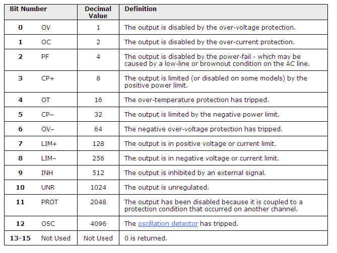
The Operation Status Group provides the normal operating modes of the power supply.  You typically want to query this register to either make sure that the power supply is either in the correct operating state or that it has completed some task (such as initiating a trigger or performing a measurement).  Here are the different members of the Operation Status Group:

 Figure 3 Operation Status Group

There are multiple ways to program using the registers.  The main way that I query the resisters is using the Condition Register.  The Condition Register will give you the real time status of the register.  Reading this register does not clear it.   A good example of using this is when you are initiating a triggered measurement:

 

INIT:ACQ (@1)                                    //This initiates the Acquire trigger system

Do

STAT:OPER:COND? (@1)       //Check the status register

               status = read

Loop Until (status And 8) = 8

*TRG  

Looking at Fig 3, 8 is the WTG_MEAS bit.  Once this is true, the unit is ready to be triggered.  This lets you make sure that you are not triggering the unit before the initiation is done.  Note that all of the statuses are referred to by the instrument by their by the bit weight (listed in the tables as the decimal value).  When you are looking for multiple statues, you need to add the bit weights.

 

The other main method of Querying the registers is using the Event register.  The Event Register is different than the Condition Register in that it keeps track of transitions in the statuses.  It does not matter when the status change happened, the Event Register will catch it and keep it until it is read back.   You do need to tell the power supply which statuses you are concerned with using the Negative Transition (STAT:OPER:NTR) and the Positive Transition (STAT:OPER:PTR) commands.  The Event Register is a latching register that will clear after it is read.  An example of using this register is when you want to make sure that there were no momentary transitions into an unwanted status.  In the following example, you want to make sure that your power supply does not go into the Unregulated mode (UNR) before you make a current measurement:

STAT:QUES:PTR 1024,(@1)            // This is the UNR bit

STAT:QUES:NTR 0, (@1)                // We are only interested in a positive transition

Body of  your program

STAT:QUES:EVEN?                        //Query the register

Status = readback

If status And 1024 =1024 then

 exit                                     //If the unit went UNR, exit

Else

                MEAS:CURR? (@1)      //measure current

                Curr=readback

End if

 

In this case, UNR is bit weight 1024.  When the unit transitions to the unregulated state (the bit transitions from 0 to 1), this bit gets set. 

As you can tell by Figure 1, there is a bunch more that you can do using status, including Service Requests but I will save those for a possible future blog post.

Please feel free to post any questions or comments here.

Some Basics on Battery Ratings and Their Validation

A key aspect of optimizing battery run-time on battery powered mobile devices is measuring and analyzing their current drain to gain greater insight on how the device is making use of its battery power and then how to make better use of it. I went into a bit of detail on this in a previous posting, “Using Current Drain Measurements to Optimize Battery Run-time of Mobile Devices”.

A second aspect of optimizing battery run-time is making certain you are making optimum use of the battery powering the device. This starts with understanding and validating the battery’s stated capacity and energy ratings. Simply assuming the battery meets or exceeds its stated ratings without validating them is bound to leave you coming up shorter than expected on run-time.  It is critical that you validate them per the manufacturer’s recommended conditions. This serves as a starting point of finding out what you can ultimately expect from the battery you intend to use in your device. More than likely constraints imposed by the nature of your device and its operating conditions and requirements will further reduce the amount of capacity you can expect from the battery in actual use.

A battery’s capacity rating is the total amount of charge the battery can deliver. It is product of the current it can deliver over time, stated as ampere-hours (Ah) or miiliampere-hours (mAh). Alternately the charge rating is also stated as coulombs (C), where:

·         1 coulomb (C)= 1 ampere-sec

·         1 ampere-hour (Ah)= 3,600 coulombs

A battery’s energy rating is the total amount of energy the battery can deliver. It is the product of the power it can deliver over time, stated as watt-hours (Wh) or milliwatt-hours (mWh). It is also the product of the battery’s capacity (Ah) and voltage (V). Alternately the energy rating is also stated as joules (J) where:

·         1 joule (J)= 1 watt-second

·         1 watt-hour (Wh) = 3,600 joules

One more fundamental parameter relating to a battery’s capacity and energy ratings is the C rate or charge (or discharge) rate. This is the ratio of the level of current being furnished (or drawn from, when discharging) the battery, to the battery’s capacity, where:

·         C rate (C) = current (A) / (capacity (Ah)

·         C rate (C) = 1 / charge or discharge time

It is interesting to note while “C” is used to designate units of C rate, the units are actually 1/h or h^-1. The type of battery and its design has a large impact on the battery’s C rate. Batteries for power tools have a high C rate capability of 10C or greater, for example, as they need to deliver high levels of power over short periods of time. More often however is that many batteries used in portable wireless mobile devices need to run for considerably longer and they utilize batteries having relatively low C rates. A battery’s capacity is validated with a C rate considerably lower than it is capable of as when the C rate is increased the capacity drops due to losses within the battery itself.

Validating a battery’s capacity and energy ratings requires logging the battery’s voltage and current over an extended period of time, most often with a regulated constant current load. An example of this for a lithium ion cell is shown in Figure 1 below. Capacity was found to be 12% lower than its rating.

Figure 1: Measuring a battery’s capacity and energy

Additional details on this can be found in a technical overview I wrote, titled “Simply Validating a Battery’s Capacity and Energy Ratings”. As always, proper safety precautions always be observed when working with batteries and cells. Validating the battery’s stated capacity and energy ratings is the first step. As the battery is impacted by the device it is powering, it must then be validated under its end-use conditions as well. Stay tuned!

Battery drain analysis of handheld HP 973A multimeter

I have owned a Hewlett-Packard 973A multimeter for longer than I can remember. What has always amazed me about this meter is that I have never had to change the batteries in it! It runs off of 2 AA batteries (in series, of course), and earlier this week, I had to open it up to change a blown fuse for the mA/uA current measurement input (that’s what I get for lending the meter to someone).

While I had it open, I took a look at the AA batteries and was surprised to see a date code of 04-99. That means these batteries have been powering this multimeter for at least 13 years! I admit that I don’t use the meter very frequently, but I am still impressed with how long these batteries lasted. The series combination measured about 2.6 V – still plenty of charge left to power the multimeter (2 new batteries in series measure about 3.2 V).

Since we make power supplies that can perform battery drain analysis, I decided to take a quick look at the current drawn by the multimeter from these batteries. I used an Agilent N6705B mainframe with an N6781A Source/Measure Unit (SMU) installed. This SMU has many features that make it easy to analyze current drain. For example, I set the SMU for Current Measure mode which means it acts like a zero-burden ammeter (an ammeter with no voltage drop across the inputs). I found that the multimeter (set to measure DC V) draws about 3.5 mA from the 2.6 V series combination of AA batteries. I used both the Meter View feature of the SMU and the Data Logger to verify the current. The Data Logger shows the dynamic current being drawn from the batteries and I measured the average current between the markers.

Typical AA batteries are rated for about 2500 mA-hours, so with a 3.5 mA load, they will last more than 700 hours. It is no wonder that the batteries lasted a long time; I use this meter only a few hours per month, so assuming 3 hours per month, the batteries would last about 20 years!

While I had the back cover off, I removed the batteries and powered the multimeter directly from the N6781A SMU. I could then slowly lower the voltage and find when the low battery indicator came on. This happened at about 2.3 V. Continuing to lower the voltage, the LCD display continued to work down to almost 1.0 V. I also noticed that the current drawn by the multimeter increased as the voltage decreased – the multimeter was drawing a nearly constant amount of power from the source – roughly 9 to 10 mW.

I figured while I had the multimeter open, I might as well install new batteries. I doubt I will write another post the next time these batteries need to be replaced in 20 to 30 years, but keep checking here.… you never know!

*OPC and You

Today I have a guest-blogger, one of my Agilent colleagues (and friends), Matt Carolan. Matt has experience with programming our power products, so I asked him if he had anything he wanted to share with our audience. He has many things to talk about and will most likely contribute to future posts, but decided to start with the *OPC command, which is the “Operation Complete” command. Here is Matt’s post:

Hi, my name is Matt and I am an Application Support Engineer at Agilent Technologies. I have had 12 years of experience programming our power products and I wanted to write about a small but powerful command, *OPC.

*OPC is a standard IEEE-488.2 command that allows you to synchronize your power supply with your program. *OPC lets you know when all pending operations are complete. A pending operation is something such as the voltage being set or the output turning on. I worked as a test engineer for a few years and we always used the *OPC command in our calibration routines. We would send a calibration command (such as CALibration:LEVel:P1) followed by a *OPC? query. This allowed us to ensure that the calibration command had finished executing and that the power supply should be outputting the correct level before we took any measurements with our test system.

    

There are two ways to use *OPC. There is a standard *OPC command and the *OPC? query. The *OPC command will set bit 0 of the Standard Event Status register when all pending operations are complete. You can then use a *ESR? Command to poll the Standard Event Status Register. When this returns a 1, all pending operations are complete. When you use this command, it only works for any pending commands that were sent BEFORE you sent the *OPC command. It will not work for commands sent after the *OPC command. You can send another *OPC command to start the cycle again.

The other way is to use it as a query. When you send a *OPC? query, it will put a 1 in the output buffer when all pending operations are complete. The main drawback of this method is that if there is an operation that takes a long time to complete, your *OPC? query will timeout. You would need to have a long timeout set in your IO library to avoid this. You cannot send any commands after the query without getting an error so this will hold up your program until all pending operations are complete.

If you have any questions please comment here or on the Agilent forum at: http://www.agilent.com/find/forums

Battery-killing cell phone apps?

Two days ago, I came across an article entitled “Do Android Security Apps Kill Your Batteries?” The article talks about mobile device users avoiding security apps because they think the apps run down their batteries too quickly. A member of the Anti-Malware Testing Standards Organization (AMTSO) is using Agilent’s N6705B DC Power Analyzer to evaluate just how much the security apps affect battery run time. While the results are not yet complete, the researchers are planning to measure power usage with no security app running, with the app running in the background, and with the app actively working. Their full report is due out by the end of July. Here is a link to the article, written by Neil Rubenking in his SecurityWatch blog for PC Magazine Digital Edition:

http://securitywatch.pcmag.com/mobile-security/298170-do-android-security-apps-kill-your-batteries

I was pleased to see the N6705B DC Power Analyzer used in this way – this product has power modules and software that are specifically designed to do exactly this type of evaluation!

If you have to evaluate a mobile device’s battery run time for any reason, here is a link to “10 Tips to Optimize a Mobile Device’s Battery Life” written by our own Ed Brorein (contributor extraordinaire to this blog):

http://cp.literature.agilent.com/litweb/pdf/5991-0160EN.pdf

And here is a link to Ed’s post from a few months ago on “Using Current Drain Measurements to Optimize Battery Run-time of Mobile Devices”:

http://powersupplyblog.tm.agilent.com/2012/03/using-current-drain-measurements-to.html

When the researchers complete and publish their evaluation on how security apps affect your cell phone battery run time, we’ll be sure to follow-up with another post! In the mean time, protect your phone in whatever way you like, and keep charging ahead by charging your batteries!

What Is Old is New Again: Soft-Switching and Synchronous Rectification in Vintage Automobile Radios

I have to admit I am a bit of a vintage electronics technologist.  One of many pass times includes bringing vintage vacuum tube automobile radios back to life. In working with modern DC sources I’ve seen innovations come about in the past decade for efficient power conversion, including soft switching and synchronous rectification. A funny thing however, for those who have been around long enough, or into vintage technologies like me, is that these issues and somewhat comparable solutions existed up to 70 years ago for automobile radios and other related electronic equipment. What is old is new again!

As we know, vacuum tubes (or valves to many) were to electronics back then as what semiconductors are to electronics today. The problem for portable and mobile equipment was that the vacuum tubes needed typically 100 or more volts DC to operate. They did have high voltage batteries for portable equipment but for automobiles the radio really needed to run off the 6 or 12 volts DC available from the electrical system. The solution: A DC/DC boost converter!

Up until the mid 1950’s most all automobile radios used vacuum tubes biased with high voltage generated from a rather primitive but clever DC/DC boost converter design. The inherent technological challenge was semiconductors did not yet exist to chop up the low-voltage, high-current DC to convert it to high-voltage, low-current DC. Of course if the semiconductors did exist this would all be a moot point! Making use of what was available the DC/DC boost converters employed what were called vibrators, which are a form of a continuously buzzing relay, to chop up the low-voltage DC for conversion. Maybe some of you are familiar with the soft humming sound heard when an original vintage automobile radio is turned on, prior to the vacuum tubes finally warming up and the audio taking over? That humming is the vibrator, the “heart” of the DC/DC boost converter in the radio.

Figure 1 below is an example circuit of vibrator-based DC/DC boost converter in a vintage automobile radio. This is just one of quite variety of different implementations created back then. Two pairs of contacts in the vibrator act in a push-pull fashion to convert the low-voltage DC into a low-voltage AC square wave. This in turn is converted to a high-voltage square wave by the transformer. Because the vibrator is an electro-mechanical device, it is limited in how fast it can switch. Switching frequencies are typically about 100 to 120 Hz. The transformers used are naturally the steel-laminated affairs similar in nature to the transformers used to convert household line voltage in home appliances. Very possibly some radio manufacturers used off- the-shelf appliance transformers in reverse to step up the voltage!  Often a small rectifier vacuum tube, such as a 6X4 (relatively modern, by vacuum tube standards) would be used to convert the high voltage AC to high voltage DC, but in this particular example I am showing here another two pairs of contacts on the secondary side switch simultaneously with the first pairs of contacts to rectify the high voltage AC. Highly efficient synchronous rectification, up to 70 years ago!

Figure 1: Representative DC/DC boost converter for a vintage automobile radio

Establishing Measurement Integration Time for Leakage Currents

The proliferation of mobile wireless devices drives a corresponding demand for components going into these devices. A key attribute of these components is the need to have low levels of leakage current during off and standby mode operation, to extend the battery run-time of the host device. I brought up the importance of making accurate leakage currents quickly in an earlier posting “Pay Attention to the Impact of the Bypass Capacitor on Leakage Current Value and Test Time”(click here to review). Another key aspect about making accurate leakage currents quickly is establishing the proper minimum required measurement integration time. I will go into factors that govern establishing this time here.

Assuming the leakage current being drawn by the DUT, as well as any bypass capacitors on the fixture, have fully stabilized, the key thing with selecting the correct measurement integration time is getting an acceptable level of measurement repeatability. Some experimentation is useful in determining the minimum required amount of time. The primary problem with leakage current measurement is one of AC noise sources present in the test set up. With DC leakage current being just a few micro amps or less these noises are significant. Higher level currents can be usually measured much more quickly as the AC noises are relatively negligible in comparison. There are a variety of potential noise sources, including radiated and conducted from external sources, including the AC line, and internal noise sources, such as the AC ripple voltage from the DC source’s output. This is illustrated in Figure 1 below. Noise currents directly add to the DC leakage current while noise voltages become corresponding noise currents related by the DUT and test fixture load impedance.

Figure 1: Some noise sources affecting DUT current measurement time

Using a longer measurement time integrates out the peak-to-peak random deviations in the DC leakage current to provide a consistently more repeatable DC measurement result, but at the expense of increasing overall device test time. Measurement repeatability should be based on a statistical confidence level, which I will do into more detail further on. Using a measurement integration time of exactly one power line cycle (1 PLC) of 20 milliseconds (for 50 Hz) or 16.7 milliseconds (for 60 Hz) cancels out AC line frequency noises. Many times a default time of 100 milliseconds is used as it is an integer multiple of both 20 and 16.7 milliseconds. This is fine if overall DUT test time is relatively long but generally not acceptable when total test time is just a couple of seconds, as is the case with most components. As a minimum, setting the measurement integration time to 1 PLC is usually the prudent thing to do when short overall DUT test time is paramount.

Reducing leakage current test time below 1 PLC means reducing any AC line frequency noises to a sufficiently low level such that they are relatively negligible compared to higher frequency noises, like possibly the DC source’s wideband output ripple noise voltage and current. Proper grounding, shielding, and cancellation techniques can greatly reduce noise pickup. Paying attention to the choice and size of bypass capacitors used on the test fixture is also important. A larger-than-necessary bypass capacitor can increase measured noise current when the measuring is taking place before the capacitor, which is many times the case. Establishing the requirement minimum integration time is done by setting a setting an acceptable statistical confidence level and then running a trial with a large number of measurements plotted in a histogram to assure that they fall within this confidence level for a given measurement integration time. If they did not then the measurement integration time would need to be increased. As an example I ran a series of trials to determine what the acceptable minimum required integration time was for achieving 10% repeatability with 95% confidence for a 2 micro amp leakage current. AC line noises were relatively negligible. As shown in Figure 2, when a large series of measurements were taken and plotted in a histogram, 95% of the values fell within +/- 9.5% of the mean for a measurement integration time of 1.06 milliseconds.

Figure 2: 2 Leakage current measurement repeatability histogram example

Leakage current measurements by nature take longer to measure due to their extremely low levels. Careful attention to minimizing noise and establishing the minimum required measurement integration time contributes toward improving the test throughput of components that take just seconds to test.