Using the Passthrough Command in IVI drivers

Hi everybody!

I was working on a customer question yesterday and I thought that it would make an enlightening blog post.  We have a feature for our IVI-COM and IVI-C drivers that allows you to directly send SCPI commands to your instrument.  This is really useful if you run into a situation where you think there is a function is missing from our driver or you run into something unexpected.  Overall, it is pretty easy to use once you know where to find it.

Let's look at the IVI-COM driver first.  You can find the passthrough in the Systems Interface under the IO property.  One you get to the IO level, you can just use the standard VISA-COM commands to send commands to the instrument and read responses back.  For my little example here I am just going to send a voltage measurement and read back the response:

In the code above, agDrvr is the name I gave to the instrument when I initialized it.

We also provide an IVI-C driver.  The IVI-C driver also has a passthrough command that is just a little more complicated than the IVI-COM version.. To send SCPI commands, you use the AgN67xx_SystemWrite function and to read data back you would use the AgN67xx_SystemRead function.  The same example as above would look like this:

In this IVI-C code:

status is where the IVI-C driver will report an error if there is an unsuccessful call 

session is the handle that I gave to this instrument when I initialized

32 was my best guess at the size of the response string.  I like to overestimate.

strResp is where I want the response to be stored

respSize is the actual size of the response and is returned by the program

All in all it's not too difficult and will definitely come in handy.  

That all I have for you this month.  As always, let us know if you have any questions.

Matt

New Keysight Power Analyzer called IntegraVision

Back on June 23, 2014, I posted about the last Agilent power products to ever be announced. At that time, we had not yet officially changed our name from Agilent to Keysight. So the AC6800 AC sources we released on that date were released under the Agilent name, soon to be rebranded to Keysight. Well, today, I am announcing the first new Keysight power product: the Keysight Technologies IntegraVision Power Analyzer Model PA2201A.

A press release went out about these products earlier today: click here to view. We here at the Power & Energy Division of Keysight have been involved in power products for decades, and of course, Keysight has an oscilloscope division with commensurate experience producing scopes. I consider the new IntegraVision power analyzers to be a combination of the vast experience of our engineers from these two disciplines combining a power analyzer and an oscilloscope. The power analyzer will enable you to accurately measure parameters such as watts, VA, VAR, power factor, crest factor, efficiency, watt-hours, amp-hours, and harmonics while the oscilloscope will allow you to visualize in real time the voltage, current, and power waveforms that are important in your design.

I am very exciting about this new line of power measurement instruments! I have been working for HP/Agilent/Keysight for nearly 35 years now and have always worked with power products during my career. One of my favorite product families to support has been the older sophisticated 6800 AC Power Source/Analyzers (not to be confused with the newer basic AC6800 series mentioned in the first paragraph above). The older AC sources can produce sine waves, square waves, and arbitrary waveforms (for tests such as cycle dropout tests) as well as measure most of the power analyzer parameters mentioned above since they have a power analyzer built into the AC source. But now the new IntegraVision power analyzer goes well beyond the capabilities of the power measurements built into our AC sources. Adding time-based measurements like watt-hours and amp-hours opens up many more energy measurement application areas for this new product and the visual waveform measurements are a huge benefit when doing things like characterizing AC inrush current or product response to AC line disturbances. I am delighted with the performance of the touch-screen on this product – it will help you gain faster insight into your designs plus it just makes using the product fun! With 0.05% basic accuracy, 5 MSample/second 16-bit digitization, and inputs isolated to 1000 V, the IntegraVision power analyzer really is a superb product for power consumption and power conversion applications. Click here for the IntegraVision web page with links to the individual products.

So the next time you need a power analyzer with great accuracy and you also want to see the power waveforms related to your application, be sure to look at Keysight’s new IntegraVision Power Analyzer Model PA2201A. I’m sure you will not be disappointed! And look here for future posts about some of the interesting applications for this product, such as AC power line disturbance measurements and micro-inverter efficiency measurements. Suggest some of your own power measurements for me to make and I’ll see what I can do for a future post for you!

A new current measurement methodology: It’s all about counting the electrons going by!

One thing near and dear to us here at the Power and Energy Division is making accurate current measurements. What exactly is current? It’s basically the flow of electric charge per unit of time. In a conductor it’s the flow of electrons through it per unit of time. 

The ampere is the fundamental unit of current in coulombs per second, which equates to 6.241x10¹⁸ electrons per second. Accurate current measurement is one of the core values of virtually all of our products. Some of the precision SMU products can measure down to femtoamp (fA) levels (10^-15 amps). This is where we tend to muse that we’re getting down to the levels where we’re virtually counting the individual electrons going by.

While there are a few different ways of measuring current, by far the most common is to measure the voltage drop across a resistive shunt. With careful design this provides the most accurate means of current measurement. There are a lot of non-obvious factors that can introduce unexpected errors that many are not aware of, leading them to believe they have better accuracy than what it really is. A good discussion of what it takes to truly make accurate current measurements was covered in a previous posting “How to make more accurate current measurements”(click here to review). We go through great pains in addressing these things in our products in order to provide accurate and repeatable measurements.

Unlike the volt and the ohm, which have quantum standards for their electrical units, the ampere instead relies on the standards for the volt and ohm for measurement, as a quantum standard for the ampere that directly relates it back to charge is still lacking. However, that may change in the not too distant future. A group of scientists were awarded the Helmholtz Prize in metrology for realization of the measurement of the ampere based on fundamental constants. Basically they’ve created an electron charge pump that moves a small, fixed quantity of electrons under control by a clock. You can say they’re literally “counting the electrons as they go by”. This could become the new SI standard reference for current measurement. To me this is very fascinating to find out about. More can be learned on this from the following link to the press release “Helmholtz Prize for the “new” ampere”(click here to review).  I am curious to see how this all plays out in the long run. Maybe it will lead to yet another, and better, way to make more accurate current measurements in products we all use today in our work in electronics!

Why is the Programming Resolution Supplemental Characteristic Listed as an Average?

Hello everyone!

Happy New Year!  This is our last post of 2014 so we wanted to wish all of our readers a Happy New Year.  Today I am going to talk about a question that I have been asked a few times lately.  In many of our power supplies, we list our Programming Resolution as an average number.  Many people want to know why we do it this way.

Look at the below snippet from our 664xA DC Power Supplies Supplemental Characteristics:

You can see that that it is clearly stated as an average.

The simple answer to this question is that this is because of calibration.

The more complex answer is that we use a DAC to control the output setting of the power supply.  A certain number of DAC counts is going to represent zero to full scale on the output of the supply.  For simplicity's sake, lets assume that we are using a 12 bit DAC for a power supply that goes to fifty volts.

In an ideal world where calibration is not necessary:
A 12 bit DAC gives us 2^12 or 4096 total counts.
The step size (programming resolution) of the 50 volt power supply would be 50/4096 or 0.0122 volts.

We do not live in an ideal world though so we have to disregard some DAC counts because of how the unit calibrates. We also generally let you program a little bit above the maximum settings (usually something like 2%).  Zero volts is not going to be zero DAC Counts and 50 V is not going to be 4096 DAC counts.  For our example, lets say that the minimum that we disregard 20 counts at the top and bottom (40 total counts) and the maximum we disregard is 120 counts (240 total counts) at the top and bottom.  In this scenario:

Minimum step size = 50/(4096-40) = 0.0123 V
Maximum step size = 50/(4096-120) = 0.0130 V

For our Supplemental Characteristic, we would take the average of those 2 numbers.   This gives us 0.01265 V.

The big question is how would I know what the programming resolution is for my particular unit.  I spent about half of yesterday trying to figure that out and I'm still working that out myself.  The best solution that I have right now is to hook a DMM to the output and slowly increment my output to see when it flips to a new setting.  I need to experiment on this though.  If any readers have a better idea, please let us know in the comments.  The fact of the matter is that the error is pretty small and to be safe, any error due to being in between DAC counts is included in our Programming Accuracy specification.

Well that is all for 2014. I hope that everyone has a safe and happy 2015.  See you next year!

Matt

Why does an electronic load draw a pulse of current when a voltage is initially applied?

We recently had a customer contact us about one of our electronic loads. He had a solid state switch in series with a fixed output voltage source (for example, 50 V) and set the load to a fixed current (for example, 1 A). He used a current probe and a scope to observe the current flowing into the electronic load. When the switch changed from open to closed he saw a pulse of current flowing into the load that was significantly higher than the load set value before the load settled to the set value of 1 A. He was wondering if this was normal. It is normal. Here’s why:

The electronic loads have a snubber network across their input terminals. The snubber typically consists of a resistor in series with a capacitor. For example, the Keysight N3304A electronic load has 2.2 uF in series with about 2 ohms. The snubber network is there to maintain stability on the load input for all settings and operating modes. When the customer’s switch was closed, the initially discharged capacitor in the snubber pulled a pulse of current to begin charging. If the dV/dt of the load input voltage waveform was infinitely fast, the cap would initially look like a short and the initial current pulse would be limited by the resistor as I = V/R. In this example, the current pulse would have been 50 V / 2 ohms = 25 A. But he was seeing a much smaller current pulse: around 2.4 A instead of 25 A, but still higher than the expected set value of 1 A. This means the dV/dt was not infinite (the solid state switch had a finite risetime). In this case, the current pulse would be limited by the dV/dt of the input voltage waveform.

As an example, see Figure 1 below showing the input voltage and input current for an N3304A load. The voltage rises from 0 V to 50 V over about 75 us and the fastest part of the risetime is about 1V/us. Since I = C dV/dt, and for this electronic load, C = 2.2 uF, the peak of the current is calculated to be 2.2 uF x 1V/us = 2.2 A. The plot shows it to be about 2.4 A, so this is close to the expected peak value. As the dV/dt of the input voltage slows down, the current drops from its peak and approaches zero amps as the dV/dt slows to zero (horizontal). (Note that in the plot below, the load was set for zero current.)

So you can see that the current flowing into the input of an electronic load may not be simply the DC setting you expect. If you apply a dynamic voltage waveform to the input, the RC snubber network will also draw some current for a short time until the voltage applied to the load input stabilizes. There is another factor involved here that is worth mentioning but I will not cover in detail in this post since it is a secondary effect in this case. In this customer’s situation, the load was set for 1 A and initially had no voltage on it (his solid state switch was open). The load was trying to draw current by turning on its input FETs, but there was no voltage applied, so the load went to an unregulated state. When the voltage finally appeared (the solid state switch was closed), the FETs that were turned on hard had to recover and take a finite amount of time to begin regulating the set current. This effect can also contribute to brief, temporary unexpected current draw by the load when a voltage is suddenly applied to the input.

Why Does Over Current Protect (OCP) have a Programmable Delay Value in the First Place?

Since I am on a roll about over current protect (OCP), having just completed a two-part posting “Why does the response time of OCP vary on the power supply I am using and what can I do about it?” (Review part 1) (Review part 2) there is yet another aspect about OCP that is worth bringing up at this time. And that is “why does OCP have a programmable delay value in the first place?” This actually came up in a discussion with a colleague here after having read my part posting.

It may seem a bit ironic that OCP has a programmable delay in that in my posting on OCP I shared ideas on how one can minimize the response time delay encountered. But this is not contradictory. One may very well want to minimize it, eliminating extra delay being encountered, but not necessarily eliminate it altogether. As can be seen in my previous postings, I had programmed the OCP delay time to 5 ms.

The programmable OCP delay does serve a purpose, and that is to prevent false OCP trips. Adding some delay time prevents these false trips.  For someone who knows the root cause of false OCP tripping they might be half right. There are actually been two main causes of false OCP trips which are prevented by adding some delay time.

The original problem with OCP was that it would be falsely tripped when output voltage settings were changed on the power supply, due to capacitive loading at the test fixture or within the DUT. This is especially prominent with inrush current when first bringing up the voltage to power the DUT. An OCP delay prevents false triggering under these conditions. To correct the false tripping the delay would be invoked when output programming changes were made. As one example, the OCP delay description in our manual for our 663x series power supplies states:

“This command sets the time between the programming of an output change that produces a constant

current condition (CC) and the recording of that condition by the Operation Status Condition register. The

delay prevents the momentary changes in status that can occur during reprogramming from being

registered as events by the status subsystem. Since the constant current condition is used to trigger

overcurrent protection (OCP), this command also delays OCP.”

Under this situation the momentary overcurrent is induced by the power supply. Although not nearly as much as in issue in practice, momentary overcurrents can also be DUT-induced as well. This is the second situation that can cause a false tripping of the OCP. The DUT may be independently turned on after the bias voltage has already been on and draw a surge of current. Or the DUT may change mode of operation and draw a temporary surge of current.  If the OCP delay is invoked only by an output programming change it does not have any effect in these situations.

On later generation products, such as our N6700, N6900, and N7900 series, the user also has the ability to programmatically select between having the OCP delay activate from either an output change, or from going into CC condition. This gives the user a way to remain consistent with original operation or have OCP delay effective for momentary DUT-induced overload currents as well!

Why does the response time of OCP vary on the power supply I am using and what can I do about it? Part 2

In the first part of this posting (click here to review) I highlighted what kind of response time is important for effective over current protection of typical DUTs and what the actual response characteristic is for a typical over current protect (OCP) system in a test system DC power supply. For reference I am including the example of OCP response time from the first part again, shown in Figure 1.

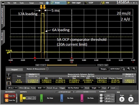
Figure 1: Example OCP system response time vs. overdrive level

Here in Figure 1 the response time of the OCP system of a Keysight N7951A 20V, 50A power supply was characterized using the companion 14585A software. It compares response times of 6A and 12A loading when the current limit is set to 5A. Including the programmed OCP delay time of 5 milliseconds it was found that the actual total response time was 7 milliseconds for 12A loading and 113 milliseconds for 6A loading.  As can be seen, for reasons previously explained, the response time clearly depends on the amount of overdrive beyond the current limit setting.

As the time to cause over current damage depends on the amount of current in excess of what the DUT can tolerate, with greater current causing damage more quickly, the slower response at lower overloads is generally not an issue.  If however you are still looking how you might further improve on OCP response speed for more effective protection, there are some things that you can do.

The first thing that can be done is to avoid using a power supply that has a full output current rating that is far greater than what the DUT actually draws. In this way the overdrive from an overload will be a greater percentage of the full output current rating. This will normally cause the current limit circuit to respond more quickly.

A second thing that can be done is to evaluate different models of power supplies to determine how quickly their various current limit circuits and OCP systems respond in based on your desired needs for protecting your DUT. For various reasons different models of power supplies will have different response times. As previously discussed in my first part, the slow response at low levels of overdrive is determined by the response of the current limit circuit.

One more alternative that can provide exceptionally fast response time is to have an OCP system that operates independently of a current limit circuit, much like how an over voltage protect (OVP) system works. Here the output level is simply compared against the protect level and, once exceeded, the power supply output is shut down to provide near-instantaneous protection. The problem here is this is not available on virtually any DC power supplies and would normally require building custom hardware that senses the fault condition and locally disconnects the output of the power supply from the DUT. However, one instance where it is possible to provide this kind of near-instantaneous over current protection is through the programmable signal routing system (i.e. programmable trigger system) in the Keysight N6900A and N7900A Advanced Power System (APS) DC power supplies. Configuring this triggering is illustrated in Figure 2.

Figure 2: Configuring a fast-acting OCP for the N6900A/N7900A Advanced Power System

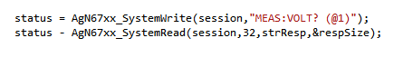
In Figure 2 the N7909A software utility was used to graphically configure and download a fast-acting OCP level trigger into an N7951A Advanced Power System. Although this trigger is software defined it runs locally within the N7951A’s firmware at hardware speeds. The N7909A SW utility also generates the SCPI command set which can be incorporated into a test program.

Figure 3: Example custom-configured OCP system response time vs. overdrive level

Figure 3 captures the performance of this custom-configured OCP system running within the N7951A. As the OCP threshold and overdrive levels are the same this can be directly compared to the performance shown in Figure 1, using the conventional, current limit based OCP within the N7951A. A 5 millisecond OCP delay was included, as before. However, unlike before, there is now virtually no extra delay due to a current limit control circuit as the custom-configured OCP system is totally independent of it. Also, unlike before, it can now be seen the same fast response is achieved regardless of having just a small amount or a large amount of overdrive.

Because OCP systems rely on being initiated from the current limit control circuit, the OCP response time also includes the current limit response time. For most all over current protection needs this is usually plenty adequate.  If a faster-responding OCP is called for minimizing the size of the power supply and evaluating the performance of the OCP is beneficial. However, an OCP that operates independently of the current limit will ultimately be far faster responding, such as that which can be achieved either with custom hardware or making use of a programmable signal routing and triggering system like that found in the Keysight N6900A and N7900A Advanced Power Systems.