Hi everybody!
I am not sure how many of you know but we have instrument specific forums at Keysight. You can find the power supply forums at: Keysight Power Supply Forums. If you have questions on power supplies you can post them there and either someone here will answer them or sometimes another user has had a similar experience.
We are also in the midst of revamping our example programs to make them more useful for our customers and would like feedback. We are interested in the following pieces of information:
1. What programming languages/IO Libraries do you use? We are thinking of concentrating on VB.NET, C#, C/C++, Labview, Matlab, Excel (VBA), and Python. Are we missing anything?
2. Any specific programming examples that would help you more effectively program your power supplies. I cannot guarantee that we will do them but anything requested will be considered.
You can either answer these questions in the comments here or you could use the forums to respond to the thread that I just created for this blog post: Power Supply Programming Example Feedback Thread.
Thanks!

Monday, August 31, 2015
Friday, August 28, 2015
Verify inverter MPPT algorithms with Keysight’s new PV array simulators
While I normally avoid simply promoting new products in my blog posts, when Keysight Technologies announces a new power product, I feel obligated to mention it here. After all, this is Keysight’s power blog!
So, yesterday, Keysight Technologies announced two new photovoltaic array simulators. Click here for the press release.


So, yesterday, Keysight Technologies announced two new photovoltaic array simulators. Click here for the press release.
The two new models are the N8937APV (208 Vac 3-phase input) and N8957APV (400 Vac 3-phase input). Both are autorangers and provide up to 15 kW, 1500 V, and 30 A on their outputs. Autoranging power supplies cover more output voltage and current combinations than power supplies with rectangular output characteristics. Click here for a previous post on autorangers and here for a post on the power supplies on which these two new models are based. These models can be put in parallel to provide a single output of up to 90 kW! They complement the family of Solar Array Simulators (SAS) that have been available from Keysight for decades.
Pictured below is the front panel of the two new photovoltaic array simulator models (15,000 W in a 3 U package):

So what is a photovoltaic array simulator? It is a specialized power supply that has an output characteristic that mimics the output characteristic of a solar panel (or a collection of solar panels known as a solar array). Photovoltaic (PV) simply refers to something that generates electricity when exposed to light so solar panels are PV devices. Solar panels have an output characteristic called an I-V curve that looks something like the solid line shown below. Isc is the short circuit current, Voc is the open circuit voltage, and Imp and Vmp are the current and voltage at the maximum power point.

Solar arrays are made by taking many solar panels and connecting them in series and parallel combinations for more power. When put in series, the total voltage increases. When put in parallel, the total current increases. Solar inverters take the DC output power from a solar array and convert it from DC into AC that can be used to power AC-mains devices (like those that plug in the wall in your home). So manufacturers of solar inverters are interested in testing their inverters and using a PV array simulator helps them. Instead of connecting their inverters to a real solar panel array that operates only when there is sunlight shining on it, they “simulate” the power output of the array with a PV array simulator. This enables them to test the inverter in many different conditions that affect the I-V curve of a solar panel, such as the temperature surrounding the panel, the angle of the sun on the panel, and cloud cover. Inverters must work when solar panels are subjected to all variations of these parameters, and waiting for them to occur with an actual solar array and the sun is not practical.
The inverter manufacturers are very interested in harvesting as much power as possible from the array, so they design their inverter circuitry to include Maximum Power Point Tracking (MPPT) algorithms that ensure their inverters operate at Pmax (the maximum power point) shown on the I-V curve above. The new Keysight photovoltaic array simulators allow engineers to test their MPPT algorithms.
So the next time you see a rooftop of solar panels, or a parking lot covered with them, or a field filled with panels collecting sunlight and converting it into electrical energy, think about the inverter connected to those panels converting the DC into AC for your use….hopefully, the inverter was fully tested with a Keysight SAS or one of these new photovoltaic array simulators!
Friday, August 14, 2015
Not all two-quadrant power supplies are the same when operating near or at zero volts!
Occasionally when working with customers on power supply
applications that require sourcing and sinking current which can be addressed
with the proper choice of a two-quadrant power supply, I am told “we need a
four-quadrant power supply to do this!” I ask why and it is explained to me
that they want to sink current down near or at zero volts and it requires
4-quadrant operation to work. The reasoning why is the case is illustrated in
Figure 1.

As can be seen in the diagram, in practical applications
when regulating a voltage at the DUT when sinking current, the voltage at the
power supply’s output terminals will be lower than the voltage at the DUT, due
to voltage drops in the wiring and connections. Often this means the power
supply’s output voltage at its terminals will be negative in order to regulate
the voltage at the DUT near or at zero volts.
Hence a four-quadrant power supply is required, right? Well,
not necessarily. It all depends on the choice of the two-quadrant power supply
as they’re not all the same! Some two-quadrant power supplies will regulate
right down to zero volts even when sinking current, while others will not. This
can be ascertained from reviewing their output characteristics.
Our N6781A, N6782A, N6785A and N6786A are examples of
some of our two-quadrant power supplies that will regulate down to zero volts
even when sinking current. This is
reflected in the graph of their output characteristics, shown in Figure 2.

Figure 2: Keysight N6781A, N6782A, N6785A and N6786A
2-quadrant output characteristics
What can be seen in Figure 2 is that these two-quadrant
power supplies can source and sink their full output current
rating, even along the horizontal zero volt axis of their V-I output
characteristic plots. The reason why they are able to do this is because
internally they do incorporate a negative voltage power rail that allows them
to regulate at zero volts even when sinking current. While you cannot program a
negative output voltage on them, making them two-quadrants instead of four,
they are actually able to drive their output terminals negative by a small
amount, if necessary. This will allow them to compensate for remote sense
voltage drop in the wiring, in order to maintain zero volts at the DUT while
sinking current. This also makes for a more complicated and more expensive
design.
Our N6900A and N7900A series advanced power sources (APS)
also have two-quadrant outputs. Their output characteristic is shown in Figure
3.

Figure 3: Keysight N6900A and N7900A series 2-quadrant
output characteristics
Here, in comparison, a certain amount of minimum positive
voltage is required when sinking current. It can be seen this minimum positive
voltage is proportional to the amount of sink current as indicated by the sloping
line that starts a small maximum voltage when at maximum sink current and
tapers to zero volts at zero sink current. Basically these series of 2-quadrant power
supplies are not able to regulate down to zero volts when sinking current.
The reason why is because they do not have an internal negative power voltage
rail that is needed for regulating at zero volts when sinking current.
So when needing to source and sink current and power near
or at zero volts do not immediately assume a 4-quadrant power supply is
required. Depending on the design of a 2-quadrant power supply, it may meet the
requirements, as not all 2-quadrant power supplies are the same! One way to
tell is to look at its output characteristics.
Thursday, July 30, 2015
How do I use Python (and no installed IO Library) to talk to my instrument?
Our newest support engineer and I have decided to learn Python (https://www.python.org/) so that we can generate programming examples. We are hearing that more and more customers are using Python so we figured that we would get on the front side and learn some Python. This blog represents my first attempts at doing anything in Python so there are probably better methods to do this but I wanted to get this out since I am pretty excited about it.
What we are going to do is do use Python with Telnet and LAN to directly send SCPI commands to my instrument. The major advantage of this is that with this method, you do not need to use an IO Library so you can use it in different operating systems. Since we are going to be using Telnet with Python, the first thing that we are going to need to do is to make sure we understand how telnet works with our power supplies. For all my work here, I will be using my N7953A Advanced Power System (APS) because it is on my desk and it is awesome. The APS uses port 5024 for telnet. On my PC running Windows 7, I enter the following in my command window:
 |
| Figure 1 |
Once I hit enter, I get our very friendly welcome screen:
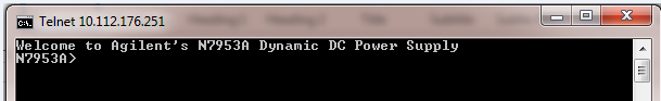 |
| Figure 2 |
Note the text “Welcome to …”, this will be important later.
To send commands or do queries, you just need to enter the
SCPI command after the prompt. The response to the query will automatically appear after you hit "Enter". Here is
how you do a *IDN? Query:
 |
| Figure 3 |
Note that the query response ends with a new line. This will be important later. The prompt also re-appears after every interaction. In the case of the APS, the prompt is the model number ("N7953A>"). On some other instruments , the prompt is "SCPI>". Either way, you need to know what the prompt is so that you can account for it later.
Now that we are Telnet experts, we are going to switch to Python and send a *IDN? query to my APS.
 |
| Figure 4 |
Basically, we are at the same point we are at in Figure 1. We essentially just hit the "Enter" key. We need to get to the equivalent to Figure 2 so that we can send a command. That means that we need to read out all of that welcome text from the power supply. Luckily, the Python Telnet Library has a read_until function that will read text until it encounters a predefined string. We know that our prompt to enter text in this case is "N6753A>" so that is what we are going to use:
 |
| Figure 5 |
Let’s send our *IDN? query. You use the write command to write to the Telnet session. Helpful tip: all commands sent through telnet
need to be terminated with a newline ("\n"):
 |
| Figure 6 |
So now that we sent a query, we need to read the buffer to get the response.
Remember that the query response ends with a
newline so we are going to use read_until and use the newline ("\n") as our read_until text:
 |
| Figure 7 |
As you can see we get the same response as before.
So now we sent our command and read the response, we need to read out the prompt again so that our power supply is ready to accept the next command sent to it. We will just use the same
read_until that we used before:
 |
| Figure 8 |
Now we are set to send the next command.
When you are done with programming the instrument, you end the Telnet session with the close command:
 |
| Figure 9 |
So that's an extremely basic example of how to use Python and Telnet. I used the shell because that is what I used to figure this all out. You can also write scripts. As Chris and I learn more about Python, we will be releasing more examples. Stay tuned for those.
Wednesday, July 29, 2015
Battery drain test on anniversary gift clock
Last month, on June 2, 2015, I celebrated working for Hewlett-Packard/Agilent Technologies/Keysight Technologies for 35 years. During the earlier times of my career, on significant anniversaries such as 10 years or 20 years, employees could choose from a catalog of gifts to have their contributions to the company recognized. That tradition has been discontinued, but I did select a couple of nice gifts over the years. During my HP days, one gift I selected was a clock with a stand shown here:
 I have had that clock for decades and it uses a silver oxide button cell battery (number 371). I have to replace the battery about once per year and wondered if that made sense based on the battery capacity and the current drain the clock presents to the battery. I expected the battery to last longer so I wanted to know if I was purchasing inferior batteries. These 1.5 V batteries are rated for about 34 mA-hours. So I set out to measure the current drain using our N6705B DC Power Analyzer with an N6781A 2-Quadrant Source/Measure Unit for Battery Drain Analysis power module installed. Making the measurement was simple…..making the connections to the tiny, delicate battery connection points was the challenging part. After one or two failed attempts (I was being very careful because I did not want to damage the connections), I solicited the help of my colleague, Paul, who handily came up with a solution (thanks, Paul!). Here is the final setup and a close-up of the connections:


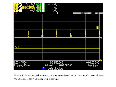
I set the N6781A voltage to 1.5 V and used the N6705B built-in data logger to capture current drawn by the clock for 5 minutes, sampling voltage and current about every 40 us. The clock has a second hand and as expected, the current showed pulses once per second when the second hand moved (see Figure 1). Each current pulse looks like the one shown in Figure 2. There was an underlying 200 nA being drawn in between second-hand movements. All of this data is captured and shown below in Figure 3 showing the full 5 minute datalog along with the amp-hour measurement (0.28 uA-hours) and average current measurement (3.430 uA) between the markers.

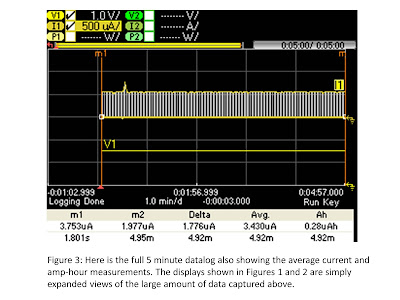 Given the average current draw, I can calculate how long I would expect a 34 mA-hour battery to last:
34 mAh / 3.430 uA average current = 9912.54 hours = about 1.13 years
This is consistent with me changing the battery about every year, so once again, all makes sense in the world of energy and electronics (whew)! Thanks to the capabilities of the N6705B DC Power Analyzer, I now know the batteries I’m purchasing are lasting the expected time given the current drawn by the clock. How much current is your product drawing from its battery?
Friday, July 24, 2015
“Adaptive Fast Charging” for faster charging of mobile devices
In some of my previous posts I have talked about USB
power delivery 2.0 providing greater power so that mobile devices can be
charged up more quickly with their USB adapters. A key part of this is these devices are
incorporating adaptive fast charging systems to accomplish faster charging. So
how does this all work anyway?
Let’s first look at the way existing USB charging work,
depicted in Figure 1.
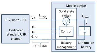
Figure 1: Legacy standard USB charging system
When the mobile device is connected to the USB adapter,
the mobile device first determines what kind of USB port it is connected to and
how much charging current is available that it will be able to draw in order to
recharge its battery. The mobile device then proceeds to internally connect its
battery up to the USB power through an internal solid state switch that
regulates the charging via the device’s internal battery management. However, a
major limitation here is the amount of available current and power. Today’s
mobile devices are using larger batteries. Up to 4 Ah batteries are commonly
used in smart phones and over 9 Ah capacity batteries are being used in
tablets. Even with later updates that increased the charging current to 1.5
amps for a dedicated charging port, this is a small fraction of the charging
current and power these larger batteries can handle. As one example, a 9 Ah
battery having a 1C recommended maximum charging rate equates to a 9 amp
charging current. This requires overnight in order to significantly recharge
the battery using standard USB charging.
The shortcomings of legacy USB for battery charging
purposes has been well recognized and the USB Power Delivery 2.0 specification
has been released to increase the amount of power available to as much as 100
watts. This is accomplished by greater voltage, up to 20 volts, and greater
current, up to 5 amps. For a mobile device incorporating this, together with an
adaptive fast charging system, is able to charge its battery in much less time.
This set up is depicted in Figure 2.

Figure 2: USB adaptive fast charging system
With adaptive fast charging, when the mobile device is
connected to the USB adapter, after determining that it has compatible fast
charging capabilities, it then negotiates for higher voltage and power. After
the negotiation the adapter then increases its output accordingly. A key thing
here is the mobile device will typically incorporate DC/DC power conversion in
its battery management system. Here it will efficiently convert the adapter’s
higher voltage charging power into greater charging current at a voltage level comparable
to the mobile device’s battery voltage, to achieve much faster charging. Now
you will be able to recharge your device over lunch instead of overnight!
Wednesday, July 15, 2015
Optimizing the performance of the zero-burden battery run-down test setup
Two years ago I added a post here to “Watt’s Up?”
titled: “Zero-burden ammeter improves battery run-down and charge
management testing of battery-powered devices” (click here to review). In this
post I talk about how our N6781A 20V, 3A 20W SMU (and now our N6785A 20V, 8A,
80W as well) can be used in a zero-burden ammeter mode to provide accurate
current measurement without introducing any voltage drop. Together with the
independent DVM voltage measurement input they can be used to simultaneously
log the voltage and current when performing a battery run-down test on a
battery powered device. This is a very useful test to perform for gaining
valuable insights on evaluating and optimizing battery life. This can also be
used to evaluate the charging process as well, when using rechargeable
batteries. The key thing is zero-burden current measurement is critical for obtaining
accurate results as impedance and corresponding voltage drop when using a
current shunt influences test results. For reference the N678xA SMUs are used
in either the N6705B DC Power Analyzer mainframe or N6700 series Modular Power
System mainframe.
There
are a few considerations for getting optimum performance when using the N678xA
SMU’s in zero-burden current measurement mode. The primary one is the way the
wiring is set up between the DUT, its battery, and the N678xA SMU. In Figure 1
below I rearranged the diagram depicting the setup in my original blog posting
to better illustrate the actual physical setup for optimum performance.

Figure
1: Battery run-down setup for optimum performance
Note that
this makes things practical from the perspective that the DUT and its battery
do not have to be located right at the N678xA SMU. However it is important that the DUT and
battery need to be kept close together in order to minimize wiring length and associated
impedance between them. Not only does the wiring contribute resistance, but its
inductance can prevent operating the N678xA at a higher bandwidth setting for
improved transient voltage response. The reason for this is illustrated in
Figure 2.

Figure
2: Load impedance seen across N678xA SMU output for battery run-down setup
The
load impedance the N678xA SMU sees across its output is the summation of the
series connection of the DUT’s battery input port (primarily capacitive), the
battery (series resistance and capacitance), and the jumper wire between the
DUT and battery (inductive). The N678xA SMUs have multiple bandwidth
compensation modes. They can be operated in their default low bandwidth mode,
which provides stable operation for most any load impedance condition. However
to get the most optimum voltage transient response it is better to operate
N678xA SMUs in one of its higher bandwidth settings. In order to operate in one
of the higher bandwidth settings, the N678xA SMUs need to see primarily
capacitive loading across its remote sense point for fast and stable operation.
This means the jumper wire between the DUT and battery must be kept short to
minimize its inductance. Often this is all that is needed. If this is not
enough then adding a small capacitor of around 10 microfarads, across the
remote sense point, will provide sufficient capacitive loading for fast and
stable operation. Additional things that should be done include:
- Place remote sense connections as close to the DUT and battery as practical
- Use twisted pair wiring; one pair for the force leads and a second pair for the remote sense leads, for the connections from the N678xA SMU to the DUT and its battery
Subscribe to:
Posts (Atom)