
Most basic performance power supplies are intended for
just providing DC power and maintain a stable output for a wide range of load
conditions. They often have lower output bandwidth to achieve this, with the
following consequences:
- Internally this means the feedback loop gain rolls off to zero at a lower frequency, providing relatively greater phase margin. Greater phase margin allows the power supply to remain stable for a wider range of loads, especially larger capacitive loads, when operating as a voltage source.
- Externally this means the output moves slower; both when programming the output to a new voltage setting as well as when recovering from a step change in output load current.
While this is reasonably suited for fairly static DC
powering requirements, greater dynamic output performance is often desirable
for a number of more demanding applications, such as:
- High throughput testing where the power supply’s output needs to change values quickly
- Fast-slewing pulsed current loads where the transient voltage drop needs to be minimized
- Applications where the power supply is used to generate power ARB waveforms
A number of things need to be done to a power supply so
that it will have faster, higher performance output response speed. Primarily
however, this is done by increasing its bandwidth, which means increasing its
loop gain and pushing the loop gain crossover out to a higher frequency. The
consequence of this the power supply’s stability can be more influenced by the
load, especially larger capacitive loads.
To better accommodate a wide range of different loads
many of our higher performance power supplies feature a programmable bandwidth
or programmable output compensation controls. This allows the output to be set
for higher output response speed for a given load, while maintaining stable
operation at the same time. As one example our N7900A series Advanced Power
System (APS) has a programmable output bandwidth control that can be set to Low, for maximum stability, or set to High1, for much greater output voltage response
speed. This can be seen in the graph in Figure 1, taken from the APS user’s
guide.
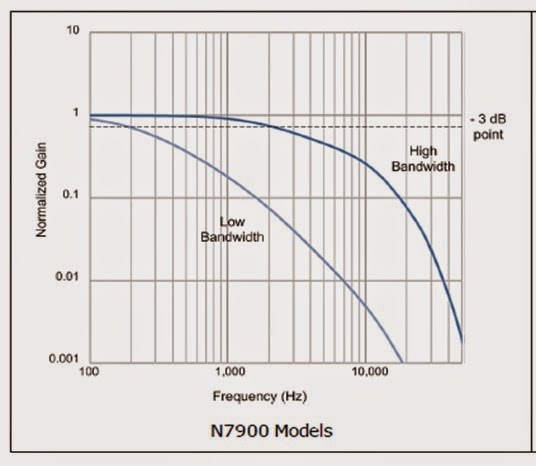
Figure 1: N7900A APS small signal resistive loading output
voltage response
Low setting
provides maximum stability and so it accommodates a wider range of capacitive
loading. High 1 setting in
comparison is stable for a smaller range of capacitive loading, but allowing
greater response bandwidth. This can be seen in table 1 below, for the
recommended capacitive loading for the N7900A APS, again taken from the APS
user’s guide.
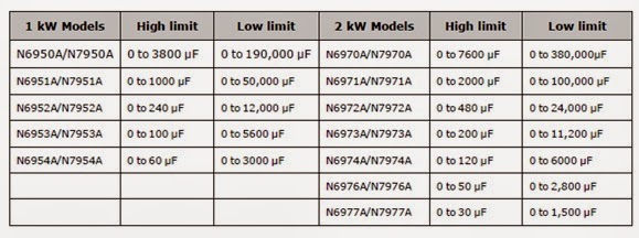
Table 1: N7900A APS recommended maximum capacitive
loading
While a maximum capacitive value is shown for each of the
different APS models for each of the two settings, this is not altogether as
rigid and fixed as it may appear. What is not so obvious is this is based on
the load remaining capacitive over a frequency range roughly comparable to the
power supply’s response bandwidth or beyond. Because of this the capacitor’s
ESR (equivalent series resistance) is an important factor. Beyond the corner
frequency determined by the capacitor’s capacitance and ESR, the capacitor
looks resistive. If this frequency is considerably lower than the power supply’s
response bandwidth, then it has little to no effect on the power supply’s
stability. This is the reason why the power supply is able to charge and
discharge a super capacitor, even though its value is far greater than the capacitance limit given, and not run into stability problems, for example.
One last consideration for more demanding applications
needing fast dynamic output changes, either when changing values or generating ARBs
is the current needed for charging and discharging capacitive loads. Capacitors increasingly become “short-circuits”
to higher AC frequencies, requiring the power supply to be able to drive or
sink very large currents in order to remain effective as a dynamic voltage
source!
.
