Eighteen months ago, in September of 2013, Keysight (we were Agilent at the time) introduced a new high-power series of power supplies: the N8900 series of 5 kW, 10 kW, and 15 kW autoranging DC power supplies. I posted about those here.
Recently, our environmental lab was doing some testing on one of the 15 kW models that required them to use a low-noise load on the output. They have electronic loads that they can connect to the output to dissipate this level of power, but to be sure they were getting the lowest noise possible, they wanted to use resistors to load the output instead of the electronic loads. Since I was amused by the size of the resistors, I thought I’d capture the moment and share a picture with you.
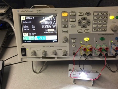
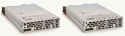
The picture shows one of our R&D engineers in our environmental lab adjusting the output voltage of a 15 kW N8900 series power supply. Notice that these power supplies pack a lot of power (15 kW) in their small 3 U high package (the white box under the fan). The four big green things on the rack are resistors. The two on the top rack are each rated for 15 kW while the two on the lower rack are each rated for 20 kW. So that’s a total of 70 kW of resistive power! Clearly, these are not your father’s ¼ W resistors!
Even with 70 kW of power dissipation capability, and “only” 15 kW available from our power supply, a big fan was needed to keep the resistors cool…..or perhaps I should say “less hot” since they still get very hot. Of course, with an extra 15 kW of power being dissipated in the room, the room temperature was going up. But that was a good thing since we are still experiencing cold weather here in New Jersey despite the fact that spring started ten days ago. So the extra heat felt good!
Before we came out with the N8900 series of high-power supplies, Matt had posted about some things around his desk that included a 2500 W resistor (click here for his post). At that time, that was a high-power resistor. But now with these 15 kW supplies, you can see we had to go much bigger! And given that these supplies can be paralleled to 100 kW or more….well….I look forward to seeing what our R&D group and environment lab engineers come up with to do resistive load testing on those. Submarine-sized resistors, perhaps? We’ll see….
Monday, March 30, 2015
Monday, March 23, 2015
Use slew rate control to cleanly power up and reduce peak inrush current of your DUTs
Previously on Watt’s Up? a colleague wrote about how the
current limit setting affects a power supply’s voltage response time (click here to review). In this posting he clearly shows how a low current limit
setting can greatly slow down the output voltage turn on response time when
powering up your DUT.
While this is generally true and good advice, especially
for basic performance power supplies, there are additional things to consider
when working with high performance power supplies models, as you will see.
Many basic performance power supplies tend to have larger
output filter capacitors in order to achieve lower output noise performance. A
disadvantage of having a large output capacitor is that it slows down the
output voltage response speed of the power supply. Basic performance power
supplies can have turn on response times on the order of a 100 milliseconds.
High performance power supplies operate by a somewhat
different set of rules. In comparison to basic performance power supplies they
typically have much smaller output capacitors and they are designed to have
output turn on and turn off response times on the order of a millisecond or
less.
However, absolute fastest is not always the best and that
is why fast, high performance power supplies also usually incorporate an output
voltage slew rate control as well. This allows you to optimize the output turn
on and turn off speed for your particular application. This lets you take
advantage of the faster output speed you have available, without it being
overkill and cause other problems.
The two most common problems that arise when powering up
and powering down many DUTs are related to charging and discharging the input
filter capacitor incorporated into them. They are:
- High peak inrush (and discharge) currents due to the high dV/dt slew rate being applied
- Power supply CC-CV mode cross over issues resulting from the high peak inrush current
To illustrate, the turn on characteristic of our N6762A
power supply was captured when powering up a load consisting of a 1,200
microfarad capacitor in parallel with a 10 ohm resistor. The N6762A was set to
10 volts and its voltage slew rate set to maximum. This was captured using the N6762A’s
digitizing voltage and current readback together with the 14585A software,
shown in Figure 1.
Figure 1: N6762A power supply turn on response set to
maximum slew rate into parallel RC load
The vertical markers have been placed at zero and maximum
voltage points of the turn on ramp. The peak inrush current reaches 3.7 amps
and the peak voltage overshoots to 11.06 volts, 10% over the 10 volt setting.
The overshoot is a result of the power supply crossing over into current limit
during the ramp up and allowing the voltage to rise to 11.06 volts before the
voltage control loop regains control to bring the output back down to 10 volts.
It also takes a little while for the voltage to settle after the peak
overshoot. Both the overshoot voltage and peak inrush current can be problems
when powering up a DUT. These occur as a result of having too fast of a voltage
slew rate when powering the DUT.
To address the problem we then set the N6762A’s slew rate
to a more acceptable value of 2,000 volts/second. The turn on voltage and
current were again captured and are shown in Figure 2. As can be seen the
voltage overshoot is eliminated and the inrush current has been reduced to a
more moderate 3.3 amps.
Figure 2: N6762A power supply turn on response set to
2,000 V/s slew rate into parallel RC load
So in closing high performance power supplies have a
significant advantage in their output response speed, in comparison to basic
power supplies. And while faster is usually better, absolute fastest may not be
best, and this applies to the output response time of power supplies as well!
But by having the ability to set the output slew rate on high performance power
supplies gives you the ability to optimize its speed for your given
application, providing for the best possible outcome possible!
.
Wednesday, March 11, 2015
Comparing effects of using pulsed and steady state power to illuminate a high brightness LED
I was having a discussion here with a colleague about the
merits of powering a high brightness LED (HBLED) using pulsed power versus
using steady state DC power.
My opinion was: “Basically, amperes in proportionally equates
to light flux out, so you will get about the same amount of illumination
whether it is pulsed or DC.”
His argument was: “Because the pulses will be brighter,
it’s possible the effective illumination that’s perceived will be brighter.
Things appear to be continuous when discrete fixed images are updated at rates
above thirty times a second, and that should apply to the pulsed illumination
as well!”
I countered: “It will look the same and, if anything,
will be less efficient when pulsed!”
So instead of continuing our debate we ran a quick
experiment. I happened to have some HBLEDs so I hooked one up to an N6781A DC
source measure module housed in an N6705B DC Power Analyzer sitting at my desk,
shown in Figure 1. The N6781A has excellent current sourcing characteristics
regardless whether it is DC or a dynamic waveform, making it a good choice for
this experiment.
Figure 1: Powering up an HBLED
First we powered it up with a steady state DC current of
100 mA. At this level the HBLED had a forward voltage drop of 2.994 V and
resulting power of 0.2994 W, as seen in Figure 2, captured using the companion
14585A control and analysis software.
Figure 2: Resulting HBLED voltage and power when powered
with 100 mA steady state DC current
We then set the N6781A to deliver a pulsed current of 200
mA with a 50% duty cycle, so that its average current was 100 mA. The results
were again captured using the 14585A software, as shown in Figure 3.
Figure 3: Resulting HBLED voltage and power when powered
with 200 mA 50% DC pulsed current
Switching back and forth between steady state DC and
pulsed currents, my colleague agreed, the brightness appeared to be comparable
(just as I had expected!). But something
more interesting to note is the average current, voltage, and power. These
values were obtained as shown in Figure 3 by placing the measurement markers
over an integral number of waveform cycles. The average current was 100 mA, as
expected. Note however that the average voltage is lower, at 2.7 V, while the
average power is higher, at 0.3127 W! At first the lower average voltage
together with higher average power would seem to be a contradiction. How can
that be?
First, in case you did not notice, the product of the RMS
voltage and RMS current are 0.3897 W which clearly does not match our average
power value displayed. What, another contradiction? Why is that? Multiplying
RMS voltage and RMS current will give you the average power for a linear
resistive load but not for a non-linear load like a HBLED. The average power
needs to be determined by taking an overall average of the power over time
computed on a point-by-point basis, which is how it is done within the 14585A
software as well as within our power products that digitize the voltage and
current over time. Second, the average voltage is lower because it drops down
towards zero during periods of zero current. However it is greater during the
periods when 200 mA is being sourced through the HBLED and these are the times
where power is being consumed.
So here, by using pulsed current, our losses ended up
being 4.4% greater when powered by the comparable steady state current. These
losses are mainly incurred as a result of greater resistive drop losses in the
HBLED occurring at the higher current level.
Saturday, February 28, 2015
Synchronize Your Measurements with Your List Transients
Hi everybody!
My blog post this month is the result of a recent customer question. The question was: how do you synchronize measurements
with list transients? The short answer
is that you use the built in digitizer to generate enough points to sample the
measurements over the entire transient. The
rest of this blog will provide the long answer.
The program that I am using here was written for a N6762A DC Power
Module but the technique will work with any power supply that has a built in
digitizer such as the Advanced Power System or any N6700 module with option
054.
For simplicity’s sake, we are going to use a 5 point
list. The voltage steps are 1 V, 2 V, 3 V,
4 V, and 5 V and the dwell times are 0.1 s, 0.2 s, 0.3 s, 0.4 s, and 0.5 s. Let’s first set the list up (please note that
all programming is done in VB.net with VISA-COM):
The next thing to do is to set up the measurement
system. We need to figure out the total
number of points that we need measure so that we can cover the entire transient. The first thing that we need to do is to
calculate the total time of the list transient (you can even do this in your
program):
The total time of our transient is 1.5 s. Now we need to use this to figure out the
number of points. I am going to choose a measurement interval of 40.96 us. This means that we want to take a measurement
every 40.96 us for 15 s. To get the
total number of points, you need to divide the total transient time by the
measurement time interval:
I’m going to round down and use 36,621
points. I’m also going to tell the power
supply to use the binary data format because as we know from my previous blog
posts, this is the fastest way to read back data. Here
is the code to set up the digitizer:
We will set our trigger source to bus for
both the transient system and the acquire system:
Next we initiate both systems:
Once the initiate is complete, we send a
trigger:
This will start both the list transient
and the digitizer. After everything is
completed, we can fetch our measured voltage array:
This array will have all of our
measurements.
I hope that this has been useful, have a
good month everyone.
Thursday, February 26, 2015
When measurements and mathematics agree, I’m happy!
I have been an electrical engineer my entire career which will span 35 years in June (yikes….I’m too young to be this old!). Despite all of that time, plus the 4 years of undergraduate study before that and 3 years to get my MSEE at night while working full time during the day, I am still amused by some simple engineering principles. When the measurements I make in the real world completely agree with the hard-core theoretical mathematics I learned in school, I am amused. Perhaps this should simply be expected (it is), but for some reason, I am still delighted when it happens. I recently had one of those simple experiences that I want to share with you today.
I was exploring some of the features on our new Keysight PA2201A IntegraVision power analyzer to better understand its operation and the applications for this new line of power measurement instrumentation. I had a simple desk lamp with a 100 W incandescent light bulb plugged into the wall outlet (120 Vac, 60 Hz here in the United States) and ran the voltage and current to the power analyzer. Given that the bulb presents a nearly pure resistive load to the sinusoidal voltage, as expected, the current was also a sine wave and in phase with the voltage. The power analyzer easily displays these measured waveforms.
What I never had an opportunity to see before was a visualization of the power waveform. For some reason, in all of my 35 years working in the power business, I never looked at a power waveform for a simple resistive load. Voltage? Sure! Current? Many times!! But power? Nope. The IntegraVision power analyzer shows voltage, current, and power waveforms as a typical display (this can be configured in quite a few other ways as well). So I was looking at the waveforms shown below.
The first thing I noticed about the power waveform was that it was sinusoidal and it never went below zero. This quickly made sense to me since I did consider the bulb to be purely resistive meaning it is consuming power 100% of the time, so all of the power flowing to the bulb had to be positive. The bulb is never pushing power back to the AC line as would happen with a reactive load especially for a purely reactive load such as a pure capacitor or inductor. If the load (the bulb) was not purely resistive, some of the power waveform would have dipped below the zero power line indicating that sometimes the load was absorbing power and sometimes it was providing power back to the line.
The next thing I noticed about the power waveform was that its phase was synchronized with the voltage and current, and it showed twice the frequency. Again, this quickly made sense since the power is simply the product of the voltage and the current [P(t) = V(t) * I(t)]. So the positive peaks have to line up (they do), the zero crossings of the voltage and current have to align with zero watts on the power waveform (they do), and the negative peaks in the voltage and current have to line up with another positive peak in the power since a negative voltage times a negative current yields a positive power (they do). This, of course, was the reason for the power waveform being twice the frequency of the voltage and current waveforms.
So I next decided to check the math behind the waveforms. I admit….I had to look up the trigonometric identity, but it was worth it! Since both the voltage and current waveforms are sine waves, and the power is the product of these, I looked up the identity for sine squared:
The voltage is a 120 Vrms, 60 Hz sine wave:
The current is 99.8 VA / Vrms = 0.832 Arms:
The power is V(t) * I(t):
Applying the above sine squared identity:
So you can see there is a 99.8 W fixed offset in the power waveform from which a cosine function is subtracted. The frequency of the cosine is 120 Hz (double the 60 Hz voltage and current waveforms). All of this completely agrees with the power waveform measured by the IntegraVision power analyzer. I am always thrilled when the math agrees with the measurements no matter how simple it is! How about you?
Labels:
IntegraVision,
PA2201A,
power analyzer,
power waveform,
sine squared,
Usage
Tuesday, February 24, 2015
Two New Keysight Source Measure Units (SMUs) for Battery Powered Device and Functional Test
Over the past few years here on “Watt’s Up?” I have
posted several articles and application pieces on performing battery drain
analysis for optimizing run time on mobile wireless devices. The key product we
provide for this application space is the N6781A 20V, +/-3A, 20W source measure
module for battery drain analysis. A second related product we offer is the
N6782A 20V, +/-3A, 20W source measure module for functional test. The N6782A
has a few less key features used for battery drain analysis but is otherwise
the same as the N6781A. As a result the N6782A is preferred product for testing
many of the components used in mobile devices, where the extra battery drain
analysis features are not needed. These products are pictured in Figure 1.
While at first glance they may appear the same, one thing to note is the N6781A
has an extra connector which is independent voltmeter input. This is used for
performing a battery run-down test, one of a number of aspects of performing
battery drain analysis. Details on these two SMUs can be found on by clicking
on: N6781A product page. N6782A product page,
Figure 1: Keysight N6781A SMU for battery drain analysis
and N6782A for functional test
These products have greatly helped customers through their
combination of very high performance specialized sourcing and measurement
capabilities tailored for addressing the unique test challenges posed by mobile
wireless devices and their components. However, things have continued to evolve
(don’t they always!). Today’s mobile devices, like smart phones, tablets and
phablets, have an amazing amount of capabilities to address all kinds of
applications. However, their power consumption has grown considerably as a
result. They are now utilizing much larger batteries to support this greater
power consumption in order to maintain reasonably acceptable battery run-time.
Optimizing battery life continues to be a critical need when developing these
products. With their higher power however, there is in turn a greater need for
higher power SMUs to power them during test and development. In response we
have just added two new higher power SMUs to this family; the N6785A 20V,
+/-8A, 80W source measure module for battery drain analysis and the N6785A 20V,
+/-8A, 80W source measure module for functional test. These products are
pictured in Figure 2. Details on these two new higher power SMUs can be found
on by clicking on: N6785A product page. N6786A product page.
Figure 2: Keysight N6785A SMU for battery drain analysis
and N6786A for functional test
A press release went out about these two new SMUs yesterday;
Click here to view. With their greater current and power capability, customers
developing and producing these advanced mobile wireless devices and their
components now have a way to test them to their fullest, not being encumbered
by power limitations of lower power SMUs.
This is exciting to me having been working within the
industry for quite some time now, helping customers increase battery life by
improving how their devices make more efficient use of the battery’s energy. A
key part of this has been by using our existing solutions for battery drain
analysis to provide critical insights on how their devices are making use of
the battery’s energy. There is a lot of innovation
in the industry to make mobile wireless devices operate with even greater
efficiency at these higher power and current levels. There is no other choice
if they are going to be successful. Likewise, it is great to see continuing to
play a key role in this trend in making it a success!
.
Labels:
battery drain analysis,
battery life,
battery run-time,
battery-powered device,
Misc.,
mobile phone,
N6705B DC Power Analyzer,
N6781A,
N6782A,
N6785A,
N6786A,
SMU,
source measure unit,
zero-burden ammeter
Monday, February 9, 2015
Consider using an electronic load for generating fast, high-power current pulses
Often there is the need for generating high-power current
pulses, typically of short duration, and having rise and fall times on the
order of microseconds. This is a common need when testing many types of power
semiconductors, for example.
When looking for a DC power supply capable of generating
very fast, high-power current pulses, one will find there are not a lot of
options readily available that are capable of addressing their needs. There are
specialized products dedicated for specific applications like this; an example
of this is Keysight’s B1505A purpose-built semiconductor test equipment. They
are capable of generating extremely fast, high-power current pulses.
Apart from specialized products however, DC power
supplies generally to not offer this kind of speed when operating in a constant
current mode (or current priority mode). One exception that comes to mind that
we provide is our N6782A and N6782A DC source measure modules. They can create
fast current pulses having just a couple of microseconds of rise and fall time.
However, they are limited to 20V, 3A, and 20W of output. Most of the higher
power, more general-purpose DC sources are not able to generate these kinds of
fast, high-power current pulses and most are really more optimized to operate
as voltage sources.
One alternative to consider for generating fast,
high-power current pulses when working with general-purpose test equipment is
to use an electronic load. You may initially say to yourself “an electronic
load is for drawing pulses of current, not sourcing them!” but when coupled to
a standard DC power supply operating as a voltage source, the setup is able to source
fast, high-power current pulses. Most electronic loads are designed to have
very fast current response. To illustrate this, I helped one customer needing
to test their high brightness LED (HBLED) arrays with fast pulses of current.
This was accomplished with the setup shown in Figure 1.
Figure 1: Load setup generating fast, high power current
pulses for LED array testing
In this setup the power supply operates as a fixed,
static voltage source. The power supply’s output voltage is set to the combined
total of the full voltage needed to drive the HBLED array at full current plus
the minimum voltage needed for the electronic load. The minimum voltage
required for the electronic load is when it conducting maximum current and most
of the power supply voltage is then applied across the HBLED array. The
electronic load’s required minimum voltage is that which supports its operation
in its linear range and maintains full dynamic response characteristics. In the
case of Keysight electronic loads this minimum voltage for linear dynamic
operation is 3 volts. Conversely the
maximum voltage required for the electronic load is when it drops down to
minimum current level, where the power supply’s voltage is instead now being
dropped across the electronic load instead of the HBLED array. Note that the
electronic load may need to maintain a very small amount of bleed current to
maintain linear operation in order to provide truly fast rise and fall times.
In this way the electronic load is able to regulate the current across the full
range with excellent dynamic response. This can be seen in Figure 2 where we were
able to achieve approximately 15 microsecond rise time right from the start.
Figure 2: Pulsed current rise time in HBLED array
One advantage of this setup is the wide range of voltage
and power that can be furnished to the DUT using a relatively low power electronic
load. A common characteristic of electronic loads is that they can dissipate a
given amount of power over an extended range of current and voltage. When the
electronic load is at maximum current it is at minimum voltage. Conversely when
it is near or at zero current it is then at its maximum voltage. In both cases
there is only a small amount of power that the electronic load needs to
dissipate. For an HBLED array it does not conduct a lot of current until it
reaches about 75% of its full operating voltage. As a result the electronic
load does not see a lot of power even on a transient basis. For this particular
situation we chose to use the Keysight N3303A 240V, 10A, 250W electronic load.
This gave a wide range of voltage, current, and power for testing a comparably wide
range of different HBLED array assemblies.
So next time you need to source fast, high-power current
pulses, you may want to think “load” instead of “source”!
Subscribe to:
Posts (Atom)