Some differences between constant current (CC) and constant resistance (CR) loading on your DUT’s performance

Most electronic loads provide constant current (CC), constant resistance (CR) and constant voltage (CV) loading. Some also offer constant power (CP) loading as well. The primary reason for this is this gives the test engineer a choice of loading that best addresses the loading requirement for the DUT, which invariably is some kind of power source.

Most usually the device should be tested with a load that reflects what the loading is like for its end use. In the most common case of a device being predominantly a voltage source the most common loading choices are either CC or CR loading, which we will look at in more detail here. Some feel they can be used interchangeably when testing a voltage source. To some extent this is true but in some cases only one or the other should be used as they can impact the DUT’s performance quite differently.

Let’s first consider static performance. In Figure 1 we have the output characteristics of an ideal voltage source with zero output resistance (a regulated power supply, for example) and a non-ideal voltage source having series output resistance (a battery, for example).  Both have the same open circuit (no load) voltage. Superimposed on these two source output characteristics are two load lines; one for CC and one for CR. As can be seen they are set to draw the same amount of current for the ideal voltage source. However, for the non-ideal voltage source, while the CC load still continues to draw the same amount of current in spite of the voltage drop, not surprisingly the CR load draws less current due to its voltage-dependent nature.

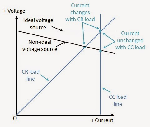
Figure 1: CC and CR loading of ideal and non-ideal voltage sources

CC loading is frequently used for static power supply tests for a key reason. Power supplies are usually specified to have certain output voltage accuracy for a fixed level of current. Using CC loading assures the loading condition is met, regardless of power supply’s output voltage being low or high, or in or out of spec. Non-ideal voltage sources, like batteries, present a little more of a problem and are often specified for both CC and CR loading as a result, to reflect the nature of the loading they may be subjected to in their end use. Due to a battery's load-dependent output voltage, trying to use one type of loading in place the other becomes an iterative process of checking and adjusting loading until the acceptable operating point is established.

Let’s now consider dynamic performance.  CC loading generally has a greater impact on a power supply’s ability to turn on as well as its transient performance and stability, in comparison to CR loading. When the power supply first starts up its output voltage is at zero. A CR load would demand zero current at start up. In comparison a CC load still demands full current. Some power supplies will not start up properly under CC loading. With regard to transient response and stability, CR loading provides a damping action, increasing current demand when the transient voltage increases and decreases demand when the transient voltage decreases, because the current demand is voltage dependent. CC loading does not do this, which can negatively influence transient response and stability somewhat. Whether CC or CR loading is used depends on what the power supply’s specifications call out for the test conditions. Batteries have some dynamic considerations as well. Their output response can be modeled as a series of time constants spanning a wide range of time. This presents somewhat of a moving target for an algorithm that uses an iterative approach to settling on an acceptable operating point.

This is just a couple of examples of how a load’s characteristic affects the performance of the device it is loading, and why electronic loads have multiple operating modes to select from, and worth giving thought next time towards how your device is affected by its loading!

Upcoming Seminar on Protecting Your Device against Power-Related Damage during Test

Here on “Watt’s Up?” we have provided a good number of posts about various protection features incorporated into system power supplies to protect your device against power-related damage during test. Just recently my colleague Gary posted “How Does Power Supply Over-Voltage Work?” (Click here to review) Here he reviews inner workings of different OVP implementations.  I recently posted “Safeguarding Your Power-Sensitive DUTs against an Over-Power Condition” (Click here to review) Here I go over a method to protect your DUT against excess power when other power supply features like over current protection may be less than ideal.

The reason why we frequently share power-related protection topics here is protecting your DUT is extremely important, there are a lot of different capabilities incorporated in system power supplies for this purpose, and there are a lot of practical considerations when putting them to use.  

Hopefully a number of you have found our posts on protection-related topics of help. Because this is a very important topic and there is so much more you should know about it I will be giving a live web-based seminar “Protecting Your Device against Power-Related Damage during Test” on August 20^th, just a few weeks away from today. I will be going over a number of protection-related topics which we have not yet covered here on “Watt’s Up?”.  One of my objectives is to provide a more holistic view of the many ways a system power supply is able to better safeguard against power-related damage as well as what is practical to expect when using these various capabilities incorporated in the power supply.

You can register online at the following (Click here for description and registration page) In case you are not able to attend the live event on August 20 you will be able to register and listen to seminar afterward as well, as it will be recorded.

So if protecting your device against power-related damage is important to you I hope you are able to attend the seminar!

Using an IVI Class Compliant Driver

Hi everybody!

In the past, I have talked about the different driver options that we offer.  One of them is the IVI-COM/IVI-C driver.  IVI actually stands for Interchangeable Virtual Instruments. Today I am going to talk about how you can make that abbreviation true using the fact that our power supply can use the IviDCPwr class.   I have received  a few questions in the past about how to do this and every time I do it, it takes me a while to remember all of the steps.  Posting it here will put it somewhere where people (including me!) can find it easily

To start off you need to download and install the following:

• The Agilent N6700 IVI-COM/IVI-C  driver from Agilent’s website.  If you get the driver from somewhere else, I am not sure how it will work.
• NI VISA since you will need NI-MAX
• IVI Compliance package

Once you have all of this, you are ready to get started.

The first thing that you need to do is set your targeted instrument in NI-MAX.  I have a N6702A connected to my LAN.  Here's how it shows up in MAX:

After that, you want to go to the "IVI-Drivers" menu, select the "Driver Sessions" item and right click on it to select "Create new".   From there, click on the "software" tab and select the appropriate driver, in this case the AgN67xx driver.  

You can see here that the driver complies to the IviDcpwr class whcih is what we will be using.  

The next thing to do is in the "Hardware" Tab of the same menu.  You need to specify which instruments use this driver.  Click on "Add" to add your instrument.  It should look like this:

 One thing that I cannot stress enough is that you need to check that checkbox.  In you don't, this will not work and you will spend a little bit of time trying to figure out why you are getting resource not found errors.  Believe me I know this from experience!  After you double check everything make sure that you click on "Save IVI Configuration".

Now choose "Logical Names".  Right click on it and select "Create New".  I created a logical name called "MPS" (this stands for Modular Power System if you were wondering).  You need to refer it to the correct driver session:

Make sure to click on "Save IVI Configuration" again.

With that, you are ready to actually start!  I used Visual C++ 2010 to write my example.  Make sure that you have all of the IVI directories properly entered in your project.  Also make sure that you reference the ividcpwr.lib file in your "linker" settings. 

Here is my program listing:

#include <stdio.h>

#include "IviDCPwr.h"

void main()

{

ViStatus status;

ViSession session;

ViRsrc resource = "MPS";

ViConstString options  = "QueryInstrStatus=true, Simulate=false, DriverSetup= Model=, Trace=false";

ViBoolean idQuery = VI_FALSE;

ViBoolean reset   = VI_TRUE;

ViBoolean enabled = VI_TRUE;

ViChar ChannelName[16] = "";

        ViInt32 index = 2;

        ViInt32 bufferSize = 256;

ViConstString Cname;

ViReal64 Vmeasurement;

ViReal64 Ameasurement;

// This program initializes a session, programs a voltage and current on channel 2, 

// enables the output, and measures voltage and current.

status = IviDCPwr_InitWithOptions(resource, idQuery, reset, options, &session);

status = IviDCPwr_GetChannelName (session,index, bufferSize,ChannelName);

Cname = ChannelName;

status = IviDCPwr_ConfigureOutputEnabled (session,Cname,enabled);

status = IviDCPwr_ConfigureVoltageLevel (session,Cname,4.0);

status = IviDCPwr_ConfigureCurrentLimit(session, Cname, IVIDCPWR_VAL_CURRENT_TRIP, 1);

status = IviDCPwr_Measure (session,Cname,IVIDCPWR_VAL_MEASURE_VOLTAGE,&Vmeasurement);

printf("Measured Voltage on channel is : %f V \n",Vmeasurement);

status = IviDCPwr_Measure (session,Cname,IVIDCPWR_VAL_MEASURE_CURRENT,&Ameasurement);

printf("Measured Current on channel is : %f A \n",Ameasurement);

status = IviDCPwr_close (session);

printf("\n Done - Press Enter to Exit");

getchar();  

}

I am not going to go over the program in detail but here are the key things to note:

• You need to include "IviDCPwr.h".  All the functions are in there.  You do not need to reference the instrument specific driver.
• When you initialize the unit, you can refer to it by the name that you define in the "Logical Names" tab above.  In my case, I use "MPS".
• This is a modular power supply.  The variable "index" is controlling the channel.  
• I have tested this program and it works properly.

In theory, you should be able to swap this power supply out with another class compliant power supply with minimal programming changes (though in this case if you switch to a single output supply you would need to take out the references to the multiple channels).

One last thing that I want to note is that this will be the last Watt's Up blog posted under the Agilent banner.  Don't worry, we will still be posting the same great content but it will be under a Keysight Technologies banner.  I have been working for Agilent for 14 years now so it will be odd at first to have a new name but I am looking forward to posting many more blogs as a Keysight employee.  Goodbye Agilent Technologies it's been an interesting 14 years!

How does power supply overvoltage protection work?

In past posts, I’ve written about what overvoltage protection (OVP) is (click here), where it is sensed (click here), and its history (click here). Today I want to cover a little about how it works inside the power supply.

As a quick review, OVP is a built-in power supply feature that protects the device under test (DUT) from excessive voltage by shutting down the power supply output if it senses voltage that exceeds the OVP setting. Depending on the power supply design, the voltage may be sensed at the output terminals or at the sense terminals.

Most of Agilent’s older power supplies sense OVP at the output terminals and use a simple analog comparator circuit to determine when the output exceeds the OVP threshold set by the user. The OVP threshold is translated into an overvoltage reference voltage (OVref) that could come from a simple divider with a potentiometer for adjustment (uncalibrated and rather crude) or from a more sophisticated calibrated digital-to-analog converter (DAC) voltage. When the comparator sees the scaled output voltage exceed the OVref voltage, the overvoltage trip (OVtrip) signal is generated which shuts down the power supply output and, on some designs, fires an SCR across the output. See Figure 1 for a simplified representation of this arrangement.

Some of our newer designs look for an overvoltage condition on the sense terminals for better accuracy. In this scheme, the sense voltage feeds one comparator input through a differential amplifier while the other comparator input is driven by the user-set calibrated OVref voltage. See Figure 2. An output terminal OVP as described above must also be used as a backup with these designs (not shown in Figure 2) because some OV conditions are not caught when sensing OV on the sense terminals. For example, if the sense leads are shorted together, the output voltage will go up uncontrolled yet the sense voltage will remain at zero volts.

Some other OVP designs use a calibrated analog-to-digital converter (ADC) on either the output terminal voltage or the sense terminal voltage and compare the measured digital data to the user’s threshold setting. See Figure 3. To avoid nuisance OVP shutdowns, this scheme frequently requires several analog-to-digital conversions in a row exceed the threshold (for example, 4). This adds a minor delay to the OVP response time. With fast ADC conversion rates, the OVP response can still be just a few tens of microseconds and it is worth spending a little extra time to gain immunity against nuisance tripping. For example, the Agilent N6781A uses this technique. Since it does an ADC conversion every 5 us and requires 4 consecutive conversions exceed the OVP threshold to cause a shutdown, it will trip in less than 30 us.

So you can see that there are various ways to implement overvoltage protection. In all cases, rest assured that your DUT is protected against excessive voltage when using Agilent power supplies!

What does it mean when my Agilent power supply displays “Osc”?

When using certain higher performance power supplies from Agilent, like the N678xA series source-measure modules, you may discover that the output has shut down and an annunciator displaying “Osc” shows up on the front panel meter display, like that shown in Figure 1 for the N6705B DC Power Analyzer mainframe. 

Figure 1: DC Power Analyzer front panel meter displaying “Osc” on channel 1 output

As you would likely guess, Osc stands for oscillation and this means the output has been shut down for an oscillation fault detection. In this particular instance an N6781A high performance source measure module was installed in channel 1 of the N6705B DC Power Analyzer mainframe.

The N678xA series source measure modules have very high bandwidth so that they can provide faster transient response and output slew rates. However, when the bandwidth of the power supply is increased, its output stability becomes more dependent on the output wiring and DUT impedances. To provide this greater bandwidth and at the same time accommodate a wider range of DUTs on the N678xA modules, there are multiple compensation ranges to select from, based on the DUT’s input capacitance, as shown in the advanced source settings screen in Figure 2.

Figure 2: DC Power Analyzer front panel displaying advanced source settings for the N678xA

Note that “Low” compensation range supports the full range of DUT loading capacitance but this is the default range. While it provides the most robust stability, it does not have the faster response and better performance of the “High” compensation ranges.

As long as the wiring to the DUT is correctly configured and an appropriate compensation range is selected the output should be stable and not trip the oscillation protection system. In the event of conditions leading to an unstable condition, any detection of output oscillations starting up quickly shut down the output in the manner I captured in Figure 3. I did this by creating an instability by removing the load capacitance.

Figure 3: Oscillation protection being tripped as captured in companion 14585A software

In rare circumstances, such as with some DUTs drawing extremely high amplitude, high frequency load currents, which may lead to false tripping, the oscillation protection can be turned off, as shown in Figure 4.

Figure 4: N678xA oscillation protection disable in N6705B DC Power Analyzer advance protection screen

Oscillation protection is a useful mechanism that can protect your DUT and your power supply from an excessively high AC voltage and current due to unstable operating conditions. Now you know what it means next time you see “Osc” displayed on the front panel of you Agilent power supply and what you need to do to rectify it!

.

Extending the usable bandwidth of the DC source when performing AC disturbance testing on your DUT

A lot of various products that run off of DC power, often destined to be used in automobiles and other types of vehicles, but even quite a number in stationary applications as well, require validation testing for impact of having AC disturbances riding on top the DC powering them.

 Conducting this type of testing is often a big challenge for the test engineer in finding a solution that adequately addresses the disturbance test requirements. It usually requires multiple pieces of hardware:

• A DC power supply is used to provide the DC bias voltage and power.
• A power amplifier is used to generate the AC disturbance.
• A separate ARB /function generator is needed to produce the reference signal for the disturbance

Coupling the DC power supply and power amplifier together is extremely problematic. While it would be great to just directly connect the two in series, this rarely can be done in practice as the power amplifier usually cannot handle the DC current of the power supply. A variety of custom approaches are then typically taken, all with their associated drawbacks.

An article about this very topic was published last year, written by a colleague I work with, Paul Young in our R&D group. As he noted it’s great when the power source can provide both the DC power as well as the AC disturbance as this is a big savings over trying to incorporate multiple pieces of equipment. Paul’s article “Extending the Usable Bandwidth of a Programmable Power Supply for Generating Sinusoidal Waveforms” (click here to review) is an excellent reference on this and the inspiration for my blog posting this week.

Our N6705B DC Power Analyzer in Figure 1 and recently introduced N7900A series Advanced Power System (APS) 1KW and 2KW power supplies in Figure 2 have proven to be very useful for doing a variety of testing where transients and audio disturbances are needing to be introduced on top of the DC that is powering the DUT.

Figure 1: Agilent N6705B DC Power Analyzer and N6700 series DC power modules

Figure 2: Agilent N7900A series 1KW and 2KW Advanced Power System and N7909A Power Dissipator

The reasons for these products being useful for disturbance testing are due to their built in ARB generation capability in conjunction with having a respectable AC bandwidth, on top of being able to source the DC power. Everything can be done within one piece of equipment.

A very common test need is to superimpose a sinusoidal disturbance in the audio range. One example of this is in automobiles. The alternator “whine” AC ripple induced on top of the DC output falls within this category. Our 1KW and 2KW N7900A series APS are good for applications needing higher DC power. However, at first glance the specified AC bandwidth of 2 kHz on does not look like it would work well for higher audio frequencies. The AC response of an N7951A from 1 kHz to 10 kHz is shown in Figure 3. This was captured using the 14585A companion software to set up its ARB.  There is noticeable roll off for higher frequency, as expected.

Figure 3: N7951A APS AC response characteristics captured using companion 14585A software

However, it’s worth noting that the roll off is gradual and very predictable. In the case of superimposing a relatively small AC signal on top of the DC output it is easy to compensate by measuring the attenuation at the given frequency and applying a gain factor to correct for it, as I did as shown in Figure 4. As one example, for 5 kHz, I programmed 2.38 volts peak to get the desired 1 volt peak.

Figure 4: N7951A APS AC response characteristics after gain correction

As can be seen it was simple to now get a flat response over the entire range. A limiting factor here is sum of the programmed DC value plus programmed AC peak value needs to be within the voltage programming range of the power supply being used. In practice, when the AC disturbance is reasonably small it is easy to cover a wide range of frequency.

Another factor to consider is capacitive loading. Some DC powered products sometimes have a fairly substantial filter capacitor built in across the DC power input. This will increase the peak current drain from the power supply when AC is applied on top of the DC. As an example a 100 microfarad capacitor will draw a peak current of 6.28 amps when a 10 kHz, 1 volt peak AC signal is applied. There may also be series impedance limiting the peak current, but whatever this AC peak current is it needs to be included when determining the size of the power supply needed.

With these basic considerations you will be able to perform AC disturbance testing over a much greater bandwidth as well!

.

Doing Inrush Current Testing with the New AC6800 AC Sources

Hi everybody,

It is the last day of the month and therefore time for me to get my blog post out.  I want to build on Gary's latest post concerning the new Agilent/Keysight AC6800 AC Sources (Click Here).  One of the key features that Gary mentioned is inrush current testing.

My colleague Russ did a video on inrush current testing for the launch.  This gives you a little bit of perspective on why you want to do the testing and gives some good tips.

When you do inrush current testing, you typically want the highest value that the current has reached when the power is enabled.  The AC6800 has a peak hold current value that will store this value for you.  The unit stores the highest current value it has measured since that value was last cleared (either manually or from power on).  One key thing to remember is to always clear out the peak hold value before doing your measurement so that you know that your measurement is up to date.

The AC6800 can synchronize the enabling of the output to a user defined phase.  When you specify the phase, it will enable the output at that phase in the sine wave (anything from 0 to 360 degrees).  The combination of the peak hold measurement and this phase synchronization are what make this testing possible.  

I  did a video for the launch where I did a tour of the front panel, including a short description of how to do inrush current testing:

  

I also have a programming example on this topic.  Below is a snippet of a program that I wrote in VB.NET using Agilent VISA-COM:

That's about it for me this month.  Please let us know if you have any questions in the comments.  

New Agilent Basic AC Power Sources

I have mentioned several times before that I avoid posting product-only-focused material in this blog, but when we announce something new, it is appropriate for me to mention it here. Today, a press release went out about our new AC sources (click here to view). You may not realize it, but this press release marks the end of an era; these are the last power products Agilent Technologies will ever announce! Now don’t go all non-linear on me…..I’m sure we will continue to design and release new power products for decades to come. But as I mentioned in a previous post (click here), as of August 1, 2014, our products will be Keysight Technologies products and not Agilent Technologies products. So these new AC sources will be rebranded to Keysight in a few weeks, but because we are releasing them before the company name change is official, we have to release them as Agilent and not Keysight. Go figure….

Anyway, what are these new Agilent (soon to be Keysight) AC sources? Well, the model numbers will remain the same through the company name change and they are:

• AC6801A (500 VA)
• AC6802A (1000 VA)
• AC6803A (2000 VA)
• AC6804A (4000 VA)

This new AC6800 Series of basic AC sources compliments our previous line of more sophisticated AC sources (click here for those) by adding lower cost models and higher power. Here is what the new series looks like (of course, the big one is the 4 kVA model):

All four new AC6800 models share these features:

• Output capabilities
• Single-phase output
• 2 ranges: 0 to 135 Vrms; 0  to 270 Vrms
• 40 Hz to 500 Hz and DC
• Sine wave (other waveforms with analog interface)
• Measurement capabilities
• Vac, Vdc, Vrms
• Iac, Idc, Irms, Ipeak, Ipeak&hold, crest factor
• Watts, VA, VAR, power factor
• Other
• Universal AC input
• LAN (LXI-Core), USB, optional GPIB
• Optional analog programming interface

The differences in the models are due to the output power ratings and can be summarized by looking at the output characteristics when producing an AC output or a DC output:

For a DC output, the graph above shows only the positive voltage and current quadrant (first quadrant). The output is equally capable of putting out negative voltage and negative current (the third quadrant) and the ratings are the same (except negative). These AC sources only source power; they cannot sink (absorb) power.

These AC sources do have one advanced feature: you can set the phase angle at which the output turns on. Coupled with the ability to measure peak current (and hold the peak current measurement), this is good for AC inrush current measurements.

To view the data sheet, click here.

So that’s the new line of basic AC power sources from Agilent and the last power products to be announced by Agilent. I wonder when the first Keysight power product announcement will be…..wouldn’t you like to know!?!?

Safeguarding your power-sensitive DUTs from an over power condition

Today’s system DC power supplies incorporate quite a variety of features to protect both the device under test (DUT) as well as the power supply itself from damage due to a fault condition or setting mishap. Over voltage protect (OVP) and over current protect (OCP) are two core protection features that are found on most all system DC power supplies to help protect against power-related damage.

OVP helps assure the DUT is protected against power-related damage in the event voltage rises above an acceptable range of operation. As over voltage damage is almost instantaneous the OVP level is set at reasonable margin below this level to be effective, yet is suitably higher than maximum expected DUT operating voltage so that any transient voltages do not cause false tripping. Causes of OV conditions are often external to the DUT.

OCP helps assure the DUT is protected against power-related damage in the event it fails in some fashion causing excess current, such as an internal short or some other type of failure. The DUT can also draw excess current from consuming excess power due to overloading or internal problem causing inefficient operation and excessive internal power dissipation.

OVP and OCP are depicted in Figure 1 below for an example DUT that operates at a set voltage level of 48V, within a few percent, and uses about 450W of power. In this case the OVP and OCP levels are set at about 10% higher to safeguard the DUT.

Figure 1: OVP and OCP settings to safeguard an example DUT

However, not all DUTs operate over as limited a range as depicted in Figure 1. Consider for example many, if not most all DC to DC converters operate over a wide range of voltage while using relatively constant power. Similarly many devices incorporate DC to DC converters to give them an extended range of input voltage operation. To illustrate with an example, consider a DC to DC converter that operates from 24 to 48 volts and runs at 225W is shown in Figure 2. DC to DC converters operate very efficiency so they dissipate a small amount of power and the rest is transferred to the load. If there is a problem with the DC to DC converter causing it to run inefficiently it could be quickly damaged due to overheating. While the fixed OCP level depicted here will also adequately protect it for over power at 24 volts, as can be seen it does not work well to protect the DUT for over power at higher voltage levels.

Figure 2: Example DC to DC converter input V and I operating range

A preferable alternative would instead be to have an over power protection limit, as depicted in Figure 3. This would provide an adequate safeguard regardless of input voltage setting.

Figure 3: Example DC to DC converter input V and I operating range with over power protect

As an over power level setting is not a feature that is commonly found in system DC power supplies, this would then mean having to change the OCP level for each voltage setting change, which may not be convenient or desirable, or in some cases practical to do. However, in the Agilent N6900A and N7900A Advance Power System DC power supplies it is possible to continually sense the output power level in the configurable smart triggering system. This can in turn be used to create a logical expression to use the output power level to trigger an output protect shutdown. This is depicted in Figure 4, using the N7906A software utility to graphically configure this logical expression and then download it into the Advance Power System DC power supply. As the smart triggering system operates at hardware speeds within the instrument it is fast-responding, an important consideration for implementing protection mechanisms.

Figure 4: N7906A Software utility graphically configuring an over power protect shutdown

A glitch delay was also added to prevent false triggers due to temporary peaks of power being drawn by the DUT during transient events. While the output power level is being used here to trigger a fault shutdown it could have been just as easily used to trigger a variety of other actions as well.

Upcoming Webinar on High Power Source/Sink Solutions for Testing Bidirectional Energy Devices

Bidirectional and regenerative energy devices both source and sink power and energy. Correspondingly, a solution that can both source and sink power and energy is needed for properly testing them. In the past here on “Watt’s up?” we have talked about what two and four quadrant operation is in our posting “What is bipolar four quadrant power? (Click here to review). We have also talked about cross over behavior between sourcing and sinking current with a DC source that will operate in two quadrants in a two-part posting  “Power supply current source-to-sink crossover characteristics” (Click here to review pt. 1) and (Click here to review pt. 2). These give useful insights about the nature of multi-quadrant solutions for bi-directional test applications.

Figure 1: The four operating quadrants

Bidirectional and regenerative energy devices that are used in many applications, such as satellite power systems, alternative energy, automotive, and many other areas, operate at kilowatt and higher power levels. These higher power levels have a significant impact on solutions and approaches taken to address their testing.  Also, the nature of these bidirectional and regenerative energy devices are not all the same. This also has an impact in that the capabilities of the test solutions need to be different to address these different types of devices.

In my upcoming webinar on June 18^th, titled “Conquering the High Power Source/Sink Test Challenge” I will be exploring the test needs of key bidirectional and regenerative energy devices and then go into the details of various test solutions and approaches for sourcing and sinking power and energy, along with their associated advantages and disadvantages. This is just a couple of weeks away. So if you are involved in this kind of work and are interested, or would just like to learn more, you can register online at the following (click here).  In case you cannot join the live event you will still be able to register and listen to seminar afterward instead, as it will be recorded.  I hope you can join in!

.

Arbs! Arbs! Arbs!

Hi everybody,

We have a new intern here and we have recently been talking about the arbitrary waveform capabilities (from now on I will refer to this as arbs)  of our power supplies and I thought that this would make an interesting blog post.  This is a really cool feature that we offer in our products as it give you the ability to create an alternating signal using our DC power supplies.  The two types of arbs are the LIST system and the constant dwell arb.

The LIST arb is a feature that we have in quite a few of our products.  The N6700 family, the N7900 family, and even some of our older power supplies have this feature.  The "Arb" system in the N6705 DC Power Analyzer is similar to the LIST.  These LISTs can contain as many as 512 different points with a timing resolution as low as 1 us.  Each point consists of a voltage or current setting and a time.  The times can be different for each point.  A short example of a programmed LIST is:

VOLT:MODE LIST
LIST:VOLT 10,25,5
LIST:DWEL 5,1,4

In the example above, the voltage will start out at 10 V and stay for 5 seconds, then transition to 25 V for 1 s and then go to 5 V for 4 s.  As you can see there are 3 voltage values with 3 corresponding dwell times.

The second mode for arbs that is only available on the N6705B DC Power Analyzer and the N7900 APS is call the Constant Dwell Arb (CD Arb).  In this mode, you can program as many as 64K points but all of the defined points have the same dwell time.  If we want to do the same waveform as above, we need to choose what will be our dwell time.  Since the smallest dwell I used in my example is 1 s, I will choose that.  Here is what a small part of the code would look like:

VOLT:MODE ARB
ARB:VOLT:CDW:DWEL 1
ARB:VOLT:CDW 10,10,10,10,10,25,5,5,5,5

The code above will produce the same waveform as the LIST example.  CD Arbs can get pretty unwieldy when you have a ton of points but we do offer some tools in our 14585A Control and Analysis software that allow you to import and export csv files to make life a bit easier.

There are advantages and disadvantages to both.  As you can see, in some cases it is easier to program a list since it requires less dwell points and gives you more flexibility with what your dwell can be.  If your waveform has a lot of DC levels in it, then the standard list might work for you.  If you have a long, complex waveform the 64 Kpoints offered in an arb will most likely offer you the best option to replicate your waveform.

Whichever arb you pick, this is a very powerful tool.  I am thinking that I will follow this up at a future date with more information about arbs.  If you have any questions, feel free to leave us some comments.

Powerlifting Agilent style!

I have been working out at a gym including lifting weights since the early 1980’s. We have a small gym here in our office building that I use a few times per week. The other day, while doing incline bench presses, my mind was wandering and I began to wonder how much power it took for me to lift the barbell and weights.

I could put the barbell and weights on a battery operated lift we have here in the office and instead of the battery, use one of our power supplies to power the lift and measure the power while operating the lift. I also wanted to calculate how much power would be required. I admit that I had to take out my old physics book to refresh my memory on how to convert weight moved through a distance to watts, but this turned out to be pretty simple: the power is just the force (weight in newtons) times the velocity. Here is the justification:

Force is mass times acceleration. F = mass*acceleration = kg-m/s^2 = newton = N which is weight when the acceleration is due to gravity (weight = mass*gravity).

Work (energy) is force (weight) applied over distance. Work = F*distance = N-m = joule = J.

Power is work per unit of time. Power = J/s = watt = W.

So power in watts = W = J/s = N-m/s = kg-m/s^2-m/s = mass * acceleration * velocity = kg*gravity*velocity = weight*velocity (gravity = 9.8 m/s^2).

During my investigation, I did go off on a tangent for a short time looking at why we talk about measuring weight in kilograms even though kilograms are units for mass and not weight. It would be proper to measure weight in newtons, not in kilograms, but that’s a different story!

So when I lift 205 lbs (93 kg) a distance of 15 inches (0.38 m) in 1.5 seconds, I use 231 watts of power to do so (mass*gravity*velocity = 93 kg * 9.8 m/s^2 * 0.38 m/1.5 s). As I mentioned above, I wanted to see if I could measure something similar with a power supply connected to a battery operated lift by using our power supplies in place of the 24 V batteries. Here is what I found:

I did a baseline power measurement of just the lift lifting some wooden pallets needed to support the barbell I was about to put on the lift. I used 2 Agilent N7972A (40 V, 50 A, 2kW) power supplies connected in parallel (I needed the extra current capacity) and set to 24 V along with our 14585A Control and Analysis Software to capture the power over time. I could then add weight and measure the incremental power required to lift the added weight.

I found that the lift itself consumes 1502 W as my baseline measurement. Then I added a 288 lb (130.6 kg) battery compartment along with 295 lbs (133.8 kg) of barbell weighs for an added 583 lbs (264.4 kg). Again, I measured the power consumed by the lift while it moved the weights vertically and found it to be 1638 W. Lifting the incremental 264.4 kg consumed an additional 136 W. Let’s see if this makes sense with a calculation. The lift moved 4.5 inches vertically in 2.2 seconds which equals 0.052 m/s. The calculated power is then 264.4 kg * 9.8 m/s^2 * 0.052 m/s = 134.7 W. That’s very close to the measured 136 W!!

It is no surprise that the laws of physics work as expected here and that our power supplies can provide insight into those laws. Agilent has added new meaning to the term “powerlifting”!

DC Source Measurement Accuracy and Resolution – With Shorter Measurement Intervals

I had gotten a customer support request a while ago inquiring about what the measurement resolution was on our new family of N6900A and N7900A Advanced Power System (APS) DC sources.  Like many of our newer products they utilize a high-speed digitizing measurement system.

 “I cannot find anything about measurement resolution in the user’s guide, it must have been overlooked!” I was told. Indeed, we have included the measurement resolution in the past on our previous products. We did not include it as a single fixed value this time around, not as an oversight however, but for good reason.

Perhaps the most correct response to the inquiry is “it depends”. Depends on what? The effective measurement resolution depends on the measurement interval that is being used. Why is that? Simply put, there is noise in any measurement system. With older and more basic products that provide low speed measurements and inherently have a long measurement interval that the voltage or current signal is integrated over, measurement system noise is usually not a big factor. However, with the higher speed digitizing measurement systems we now employ in our performance DC sources, factoring in noise based on the measurement interval provides a much more realistic and meaningful answer.

For the N6900A and N7900A APS products we include Table 1 shown below, in our user’s guide to help customers ascertain what the measurement accuracy and resolution is, based on the measurement interval (i.e. measurement integration period) being used is.

  

Table 1: N6900A/N7900A measurement accuracy and resolution vs. Measurement interval

This table is meant to provide an added error term when using shorter measurement intervals. We use 1 power line cycle (1 NPLC) as the reference point at the top of the table, for the measurement accuracy provided in our specifications. This is a result of averaging 3,255 single samples together. By doing this we have effectively spread the measurement system noise over a greater band and filtered it out by the averaging. For voltage measurements the effective resolution is over 20 bits.

Note now at the bottom of the table there is the row for one point averaged. It is for 0.003 NPLCs, which is 5 microseconds, the sampling period of the digitizer in our DC source. For a single sample the effective measurement resolution is now 12.3 bits for voltage. Note also we provide an accuracy error adder term of 0.02%. This is taking into account the measurement repeatability affecting the accuracy.

A convenient expression for converting from number of bits to dB of signal to noise (SNR) for a digitizer is given by:

SNR (dB) = 6.02 x n (# of bits) + 1.76

The 12.3 bits of effective resolution equates to 75.8 dB of SNR, which is very much in line with what to expect from a wide band, high speed digitizing measurement system like what is provided in this product family.

As previously mentioned the effective measurement resolution is over 20 bits for a 1 NPLC measurement interval. This actually happens to be greater than the actual ADC used. While there is less resolution when using shorter measurement intervals, conversely greater resolution can be achieved by using longer measurement intervals, which I expect to talk more about in a future posting here on “Watt’s Up?”!

In the meantime this is just one more example of how we’re trying to do a better job specifying our products to make them more useful and applicable in ascertaining what their true performance will be in one’s end application.

European Space Power Conference (ESPC) for 2014

This week’s blog posting is going in a bit of a different direction, as I likewise did last month, to attend and participate in the 2014 European Space Power Conference (ESPC) for 2014. While this was the tenth ESPC, which I understand takes place every couple of years; this was the first time I had opportunity to attend. One thing for certain; this was all about DC power, which is directly aligned with the things I am always involved in. In this particular instance it was all about DC power for satellites and space-bound crafts and probes.

I initially found it just a bit curious that a number of the keynote speeches also focused a fair amount on terrestrial solar power as well, but I supposed I should not be at all surprised. There has been a large amount of innovation and a variety of things that benefit our daily lives that came out of our own space program, fueled by our involvement in the “space race” and still continuing on to this day. (Can you name a few by chance?). This is a natural progression for a vast number of technological advances we enjoy.

At ESPC there were numerous papers presented on solar cells and arrays, batteries and energy storage, nuclear power sources, power conversion and DC/DC converters, super-capacitors, and a variety of other topics related to power. Just a couple of my learnings and observations include:

·         There was a very high level of collaboration of sharing findings and answering questions among peers attending the event

·         While batteries generally have very limited lives, from findings presented, it was interesting to see how well they have performed over extended periods in space, lasting last well in excess of their planned life expectancies. It is a reflection of a combination of several things including careful control and workmanship, understanding life-shortening and failure mechanisms, how to take properly treat them over time, what should be expected, as well as other factors contributing to their longevity. I expect this kind of work will ultimately find its way to being applied to using lithium ion batteries in automotive as well.

·         A lot of innovation likewise continues with solar cell development with higher conversion efficiencies coming from multi-junction devices. Maybe we’ll see this become commonplace for terrestrial applications before long!

·         A number of research papers were presented from participants from universities as well. In all, the quality of work was excellent.

I was there with another colleague, Carlo Canziani. Together we represented some of our DC power solutions there, including our N7905A DC Power Analyzer, N7900 series Advanced Power System (APS), and E4360A series Solar Array Simulator (SAS) mainframe and modules. These are the kinds of advanced power stimulus and measurement test instruments vital for conducting testing on satellite and spacecraft power components and systems.

In all it was a refreshing change of pace to be at an event where power is the primary focus, and if this happens to be an area of interest to you as well, you can find out more about ESPC from their site by clicking on the following link: (ESPC2014). Maybe you will find it worthwhile to attend or even present results of some of your work at the next one as well!

New Software Update for the N7900 Advanced Power System

Hi everybody,

Last year, we introduced the Agilent N7900 Advanced Power System (hereon in shortened to N7900 APS).  The N7900 APS is a full of great features that can only be accessed using the instrument's programming interface.  The programming interface works very well but sometimes you just don't want write and troubleshoot a program, you just want something that works.

Well, I have the chance to share some pretty exciting news.  We want to provide you software that makes some of these great features easy for you to use.  The software is the 14585A Control and Analysis Software.  This software was previously only available for the N6705 DC Power Analyzer.

The 14585A software is a standalone application that unlocks three key features: it allows you to look at a graphical representation of the measured data in Scope Mode, create arbitrary waveforms in Arb mode, and log long term data in datalogger mode.  These three advanced features can be setup and run by adjusting a few settings and pressing a few buttons.

 The software comes with a 30 day free trial so feel free to download it to check it out.  Please note that you need at least version A.01.13 of the APS firmware in order to use the software.

You can find the latest APS firmware at:
APS Firmware

You can find the software at:
14585A Software

If you have any questions on the software, feel free to leave us some comments.  Thanks for reading!

Measurement of AC plus DC voltage

One of our AC source customers recently asked me to justify the reading on the front panel of one of our AC sources set to produce a sine wave with a DC offset. He had our 6812B AC Power Source/Analyzer set to a sine wave of 100 Vac (60 Hz) and added a DC offset of 50 Vdc. These AC sources can produce output voltages of up to 300 Vrms and DC voltages up to +/- 425 Vdc. With his settings of 100 Vac and 50 Vdc, the front panel meter was reading 111.79 V with the meter set to measure AC+DC. At first this seemed like an odd result to me, but then I realized that we are simply measuring the rms (root-mean-square) of the total waveform (AC plus DC) and that should be the square-root of the sum-of-the-squares of the individual rms values. This can be mathematically proven fairly easily. Since the AC source Vac is set in rms volts and the rms of DC is simply the DC voltage:

This works even if the DC value is set to -50 Vdc instead of +50 Vdc since the value is squared. And sure enough, when I set the AC source output to 100 Vac and -50 Vdc, the front panel measurement shows 111.82 as expected. The small variation in the measured value compared to the exact calculated value is due to the slight inaccuracies in both the output setting and measurement system.

So in summary, measurement of an rms waveform that consists of an AC signal plus a DC signal is the square-root of the sum-of-the-squares of the individual two values. It’s as simple as that!

Upcoming Seminar on Using Your Power Supply to Improve Test Throughput

I have provided here on “Watt’s up?” a number of ideas on how you can improve your test throughput from time to time, as it relates on how to make better use of you system power supplies to accomplish this. I have categorized these ideas on how to improve throughput as either fundamental or advanced.

In “How fundamental features of power supplies impact your test throughput” (click here to review) I shared in a two-part posting definitions of key fundamental power supply features that impact test throughput and ways to make improvements to literally shave seconds off of your test time.

One example (of several) of an advanced idea on improving throughput I previously shared here is “Using the power supply status system to improve test throughput” (click here to review). Here I explain how, by monitoring the status system, you can improve throughput by not relying on using excessively long fixed wait statements in your programming.

I hope you have found these ideas helpful. If you would like to learn more about using your system power supply to improve your test throughput I will be presenting a live web-based seminar this week, in just a couple of days, April 30^th, at 1:00 PM EST on this very topic!

In this seminar I will go through a number of things I’ve shared here on “Watt’s up?” in the past, but in greater detail. In addition, I have also prepared several new ideas as well in this seminar that you might find of help for your particular test situation.  You can register online at the following (click here to access seminar description and registration).  In case you miss the live event I expect you will be able to register and listen to seminar afterward as well, as it will be recorded.

So if improving your test throughput is important to you I hope you are able to attend the seminar!

Why have programmable series resistance on a power supply’s output?

A feature we’ve included on our 663xxA Mobile Communications DC Sources, our N6781A 2-quadrant Source Measure Module, and most recently our N69xxA and N79xxA Advanced Power System (APS) is the ability to program in a value for a resistance that exists in series with the output voltage. So why do we offer this?

 Batteries are not ideal voltage sources. They have a significant amount of equivalent series resistance (ESR) on their output. Because of this, the battery’s output has a voltage drop that is proportional to the current drawn by the DUT that is being powered. An example of this is shown in the oscilloscope capture in Figure 1, where a GPRS mobile handset is drawing pulsed transmit current from its battery.

Figure 1: Battery voltage and current powering a GPRS handset during transmit

In comparison, due to control feedback, a conventional DC power supply has extremely low output impedance. At and near DC, for all practical purposes, the DC output resistance is zero. At the same time, during fast load current transition edges, many conventional DC power supplies can have fairly slow transient voltage response, leading to significant transient overshoots and undershoots with slow recovery during these transitions, as can be seen in the oscilloscope capture in Figure 2.

Figure 2: Example general purpose bench power supply powering a GPRS handset during transmit

It’s not hard to see that the general purpose bench power supply voltage response is nothing close to that of the battery’s voltage response and recognize that it will likely have a significant impact on the performance of the GPRS handset. Just considering the performance of the battery management, the battery voltage drop during loading and rise during charging, due to the battery’s resistance, will impact discharge and charge management performance.

We include programmable resistance in the above mentioned DC power supplies as they are battery simulators.  By being able to program a series output resistance these power supplies are able to better simulate the voltage response of a battery, as shown in Figure 3.

Figure 3: N6781A battery simulator DC source powering a GPRS handset during transmit

While the 663xxA and N6781A are fairly low power meant to simulate batteries for handheld mobile devices, The N69xxA and N79xxA APS units are 1 and 2 KW power supplies meant to simulate much larger batteries used in things like satellites, robotics, regenerative energy systems, and a number of other higher power devices. Figure 4 shows the voltage response of an N7951A 1 KW APS unit programmed to 20 milliohms output impedance, having a +/- 10 amp peak sine wave load current applied to its output.

Figure 4: N7951A 1 KW APS DC source voltage response to sine wave load

Programmable series output resistance is one more way a specialized DC source helps improve performance and test results, in this case doing a better job simulating the battery that ultimately powers the device under test.

Use the FETCH Command to Minimize Your Measurement Time

Hi everyone,

I am back again with another programming tip for you.  A neat feature on some of our products that many people many not know about is the ability to fetch measurements from a previous acquisition.  Quite a few of our power supplies and loads (the N6700 modules, the N7900 APS power supplies, the 681xB AC Sources, the N3300 loads, and probably some others that I am probably forgetting) have the ability to acquire voltage and current measurements at the same time.  This is done using the FETCH command (in my little example snippets I use the SCPI short form of FETC).  In a previous blog post I used this command to read back an array of current measurements (see Inrush Current Measurements).  In that command, I use a FETCH command to retrieve a triggered measurement.  

There is another, very useful way to use the FETCH commands.  I am not really sure what the best way to phrase it so I am going to take a shot and then illustrate with an example.  When you send a measure command (say for voltage), the measurement system will also acquire the other measurement (in this case current) and you can send a FETCH command to retrieve that acquired data.   Here is a very small example with some comments (all these commands tested on a N7952A Advanced Power System):

Example Snippet 1:
MEAS:VOLT? -> This will start a new acquisition and take the measurements 
<read back the voltage measurement data>
FETC:CURR? -> This will return the current measured during the voltage measurement above
<read back fetched current measurements>

Since we have voltage and current measurements, the instrument can calculate power:
FETC:POW? -> P=V*I
<read back calculated power>

Please note that you can do this with arrays as well. 

How can this save me time in my program you ask?  Well these power supplies all have built in digitizers that you can access with some programming commands.  The default measurement (at 60 Hz line frequency) is 3255 points measured at 5.12 us per point.  That is a total measurement time of  16.67 ms.  You have the ability to change this to fit your needs though.  You can measure up to 512 Kpoints at up to 40,000 s per point.  Every time you send a measure command you need to wait for the measurement to complete.  For instance:

Example Snippet 2:
MEAS:VOLT?
<read back the voltage measurement data> 
MEAS:CURR? 
<read back the current measurement data>

You will need to wait for two acquisition periods because you are initiating two separate measurements.  In the first example snippet, only the MEAS:VOLT? is initiating a measurement, the FETC:CURR is just reading data out of the instrument.    The downside is that the data that you fetch is going to be of the same age as the last measurement you did so if you need something newer, you need to do a new measurement.  Overall though I think that FETCH is a very useful command.  

I hope people find this useful.  Let us know if you have any questions by using the comments.  

What is a floating power supply output?

First let me tell you that a floating power supply output is NOT what is shown below in Figure 1 (haha).

Now some background: earth ground is the voltage potential of the earth and to greatly reduce the risk of subjecting a person to an electrical shock, the outer covering (chassis) of most electrical devices is internally connected to a wire that is connected to earth ground usually through the power cord. The idea here is to ensure that all surfaces a person can touch are at the same voltage potential; namely, the one that he is standing on: earth ground. As long as that is true, the person can freely touch things without the risk of getting shocked due to two of the things he touches at the same time being at different voltage potentials, or one of the things being at a high voltage potential with respect to the earth. If the voltage difference is high enough, the person could be shocked. Earth grounding the chassis also protects the user if there is an internal problem with an electrical device causing its chassis to inadvertently come in contact with an internal high voltage wire. Since the chassis is earth grounded, an internal short to the chassis is really a short to ground and will blow a fuse or trip a circuit breaker to protect the user instead of putting the chassis at the high voltage. If you touched a chassis that had a high voltage with respect to ground on it, your body completes the path to ground and you get shocked!

So to protect the user (and for some other reasons), the chassis of Agilent power supplies are grounded internally through the ground wire (the third wire) in the AC input line cord. Additionally, most if not all of our Agilent power supplies have isolated (floating) outputs. That means that neither the positive output terminal nor the negative output terminal is connected to earth (chassis) ground. See Figure 2.

Figure 3 shows an example of non-floating outputs with the negative output terminal grounded.

For floating DC power supplies, the voltage potential appears from the positive output terminal to the negative output terminal. There is no voltage potential (at least, none with any power behind it) from either the positive terminal to earth ground or from the negative output terminal to earth ground. A power supply with a floating output is more flexible since, if desired, either the positive or negative terminal (or neither) can be connected to earth ground. Some devices under test (DUT) have a DC input with either the positive or negative input terminal connected to earth ground. If one of the power supply outputs was also internally connected to earth ground, when connected to the DUT, it could short out the power supply output. So power supplies with floating output terminals (no connections to earth ground) are more versatile.

If the outputs are floating from earth ground, we need to specify how far above or below earth ground you can float the output terminals. Our power supply documentation provides this information. For example, most Agilent power supply output terminals can float to +/-240 Vdc off of ground. You will frequently see the following in our documentation:

Also, some power supplies have different float ratings for the positive and negative output terminals. For example, for Agilent N5700 models rated for more than 60 Vdc, the following note in the manual means you can float the positive output terminal up to +/-600 Vdc from ground or the negative output terminal up to +/-400 Vdc from ground:

The output characteristic table may list this as “Output Terminal Isolation” as shown below which means the same thing as maximum float voltage:

Figure 4 shows an example of floating a power supply to 200 V above ground. The power supply output is set to 40 V.

You can see from the last example that you have to take the power supply output voltage into consideration when ensuring you are not violating the float voltage rating. If you exceed the float voltage rating of the power supply, you are potentially exceeding the voltage rating of internal parts that could cause the internal parts to fail or break down and present a shock hazard, so don’t violate the float voltage rating!