Upcoming Webinar on High Power Source/Sink Solutions for Testing Bidirectional Energy Devices

Bidirectional and regenerative energy devices both source and sink power and energy. Correspondingly, a solution that can both source and sink power and energy is needed for properly testing them. In the past here on “Watt’s up?” we have talked about what two and four quadrant operation is in our posting “What is bipolar four quadrant power? (Click here to review). We have also talked about cross over behavior between sourcing and sinking current with a DC source that will operate in two quadrants in a two-part posting  “Power supply current source-to-sink crossover characteristics” (Click here to review pt. 1) and (Click here to review pt. 2). These give useful insights about the nature of multi-quadrant solutions for bi-directional test applications.

Figure 1: The four operating quadrants

Bidirectional and regenerative energy devices that are used in many applications, such as satellite power systems, alternative energy, automotive, and many other areas, operate at kilowatt and higher power levels. These higher power levels have a significant impact on solutions and approaches taken to address their testing.  Also, the nature of these bidirectional and regenerative energy devices are not all the same. This also has an impact in that the capabilities of the test solutions need to be different to address these different types of devices.

In my upcoming webinar on June 18^th, titled “Conquering the High Power Source/Sink Test Challenge” I will be exploring the test needs of key bidirectional and regenerative energy devices and then go into the details of various test solutions and approaches for sourcing and sinking power and energy, along with their associated advantages and disadvantages. This is just a couple of weeks away. So if you are involved in this kind of work and are interested, or would just like to learn more, you can register online at the following (click here).  In case you cannot join the live event you will still be able to register and listen to seminar afterward instead, as it will be recorded.  I hope you can join in!

.

Arbs! Arbs! Arbs!

Hi everybody,

We have a new intern here and we have recently been talking about the arbitrary waveform capabilities (from now on I will refer to this as arbs)  of our power supplies and I thought that this would make an interesting blog post.  This is a really cool feature that we offer in our products as it give you the ability to create an alternating signal using our DC power supplies.  The two types of arbs are the LIST system and the constant dwell arb.

The LIST arb is a feature that we have in quite a few of our products.  The N6700 family, the N7900 family, and even some of our older power supplies have this feature.  The "Arb" system in the N6705 DC Power Analyzer is similar to the LIST.  These LISTs can contain as many as 512 different points with a timing resolution as low as 1 us.  Each point consists of a voltage or current setting and a time.  The times can be different for each point.  A short example of a programmed LIST is:

VOLT:MODE LIST
LIST:VOLT 10,25,5
LIST:DWEL 5,1,4

In the example above, the voltage will start out at 10 V and stay for 5 seconds, then transition to 25 V for 1 s and then go to 5 V for 4 s.  As you can see there are 3 voltage values with 3 corresponding dwell times.

The second mode for arbs that is only available on the N6705B DC Power Analyzer and the N7900 APS is call the Constant Dwell Arb (CD Arb).  In this mode, you can program as many as 64K points but all of the defined points have the same dwell time.  If we want to do the same waveform as above, we need to choose what will be our dwell time.  Since the smallest dwell I used in my example is 1 s, I will choose that.  Here is what a small part of the code would look like:

VOLT:MODE ARB
ARB:VOLT:CDW:DWEL 1
ARB:VOLT:CDW 10,10,10,10,10,25,5,5,5,5

The code above will produce the same waveform as the LIST example.  CD Arbs can get pretty unwieldy when you have a ton of points but we do offer some tools in our 14585A Control and Analysis software that allow you to import and export csv files to make life a bit easier.

There are advantages and disadvantages to both.  As you can see, in some cases it is easier to program a list since it requires less dwell points and gives you more flexibility with what your dwell can be.  If your waveform has a lot of DC levels in it, then the standard list might work for you.  If you have a long, complex waveform the 64 Kpoints offered in an arb will most likely offer you the best option to replicate your waveform.

Whichever arb you pick, this is a very powerful tool.  I am thinking that I will follow this up at a future date with more information about arbs.  If you have any questions, feel free to leave us some comments.

Powerlifting Agilent style!

I have been working out at a gym including lifting weights since the early 1980’s. We have a small gym here in our office building that I use a few times per week. The other day, while doing incline bench presses, my mind was wandering and I began to wonder how much power it took for me to lift the barbell and weights.

I could put the barbell and weights on a battery operated lift we have here in the office and instead of the battery, use one of our power supplies to power the lift and measure the power while operating the lift. I also wanted to calculate how much power would be required. I admit that I had to take out my old physics book to refresh my memory on how to convert weight moved through a distance to watts, but this turned out to be pretty simple: the power is just the force (weight in newtons) times the velocity. Here is the justification:

Force is mass times acceleration. F = mass*acceleration = kg-m/s^2 = newton = N which is weight when the acceleration is due to gravity (weight = mass*gravity).

Work (energy) is force (weight) applied over distance. Work = F*distance = N-m = joule = J.

Power is work per unit of time. Power = J/s = watt = W.

So power in watts = W = J/s = N-m/s = kg-m/s^2-m/s = mass * acceleration * velocity = kg*gravity*velocity = weight*velocity (gravity = 9.8 m/s^2).

During my investigation, I did go off on a tangent for a short time looking at why we talk about measuring weight in kilograms even though kilograms are units for mass and not weight. It would be proper to measure weight in newtons, not in kilograms, but that’s a different story!

So when I lift 205 lbs (93 kg) a distance of 15 inches (0.38 m) in 1.5 seconds, I use 231 watts of power to do so (mass*gravity*velocity = 93 kg * 9.8 m/s^2 * 0.38 m/1.5 s). As I mentioned above, I wanted to see if I could measure something similar with a power supply connected to a battery operated lift by using our power supplies in place of the 24 V batteries. Here is what I found:

I did a baseline power measurement of just the lift lifting some wooden pallets needed to support the barbell I was about to put on the lift. I used 2 Agilent N7972A (40 V, 50 A, 2kW) power supplies connected in parallel (I needed the extra current capacity) and set to 24 V along with our 14585A Control and Analysis Software to capture the power over time. I could then add weight and measure the incremental power required to lift the added weight.

I found that the lift itself consumes 1502 W as my baseline measurement. Then I added a 288 lb (130.6 kg) battery compartment along with 295 lbs (133.8 kg) of barbell weighs for an added 583 lbs (264.4 kg). Again, I measured the power consumed by the lift while it moved the weights vertically and found it to be 1638 W. Lifting the incremental 264.4 kg consumed an additional 136 W. Let’s see if this makes sense with a calculation. The lift moved 4.5 inches vertically in 2.2 seconds which equals 0.052 m/s. The calculated power is then 264.4 kg * 9.8 m/s^2 * 0.052 m/s = 134.7 W. That’s very close to the measured 136 W!!

It is no surprise that the laws of physics work as expected here and that our power supplies can provide insight into those laws. Agilent has added new meaning to the term “powerlifting”!

DC Source Measurement Accuracy and Resolution – With Shorter Measurement Intervals

I had gotten a customer support request a while ago inquiring about what the measurement resolution was on our new family of N6900A and N7900A Advanced Power System (APS) DC sources.  Like many of our newer products they utilize a high-speed digitizing measurement system.

 “I cannot find anything about measurement resolution in the user’s guide, it must have been overlooked!” I was told. Indeed, we have included the measurement resolution in the past on our previous products. We did not include it as a single fixed value this time around, not as an oversight however, but for good reason.

Perhaps the most correct response to the inquiry is “it depends”. Depends on what? The effective measurement resolution depends on the measurement interval that is being used. Why is that? Simply put, there is noise in any measurement system. With older and more basic products that provide low speed measurements and inherently have a long measurement interval that the voltage or current signal is integrated over, measurement system noise is usually not a big factor. However, with the higher speed digitizing measurement systems we now employ in our performance DC sources, factoring in noise based on the measurement interval provides a much more realistic and meaningful answer.

For the N6900A and N7900A APS products we include Table 1 shown below, in our user’s guide to help customers ascertain what the measurement accuracy and resolution is, based on the measurement interval (i.e. measurement integration period) being used is.

  

Table 1: N6900A/N7900A measurement accuracy and resolution vs. Measurement interval

This table is meant to provide an added error term when using shorter measurement intervals. We use 1 power line cycle (1 NPLC) as the reference point at the top of the table, for the measurement accuracy provided in our specifications. This is a result of averaging 3,255 single samples together. By doing this we have effectively spread the measurement system noise over a greater band and filtered it out by the averaging. For voltage measurements the effective resolution is over 20 bits.

Note now at the bottom of the table there is the row for one point averaged. It is for 0.003 NPLCs, which is 5 microseconds, the sampling period of the digitizer in our DC source. For a single sample the effective measurement resolution is now 12.3 bits for voltage. Note also we provide an accuracy error adder term of 0.02%. This is taking into account the measurement repeatability affecting the accuracy.

A convenient expression for converting from number of bits to dB of signal to noise (SNR) for a digitizer is given by:

SNR (dB) = 6.02 x n (# of bits) + 1.76

The 12.3 bits of effective resolution equates to 75.8 dB of SNR, which is very much in line with what to expect from a wide band, high speed digitizing measurement system like what is provided in this product family.

As previously mentioned the effective measurement resolution is over 20 bits for a 1 NPLC measurement interval. This actually happens to be greater than the actual ADC used. While there is less resolution when using shorter measurement intervals, conversely greater resolution can be achieved by using longer measurement intervals, which I expect to talk more about in a future posting here on “Watt’s Up?”!

In the meantime this is just one more example of how we’re trying to do a better job specifying our products to make them more useful and applicable in ascertaining what their true performance will be in one’s end application.

European Space Power Conference (ESPC) for 2014

This week’s blog posting is going in a bit of a different direction, as I likewise did last month, to attend and participate in the 2014 European Space Power Conference (ESPC) for 2014. While this was the tenth ESPC, which I understand takes place every couple of years; this was the first time I had opportunity to attend. One thing for certain; this was all about DC power, which is directly aligned with the things I am always involved in. In this particular instance it was all about DC power for satellites and space-bound crafts and probes.

I initially found it just a bit curious that a number of the keynote speeches also focused a fair amount on terrestrial solar power as well, but I supposed I should not be at all surprised. There has been a large amount of innovation and a variety of things that benefit our daily lives that came out of our own space program, fueled by our involvement in the “space race” and still continuing on to this day. (Can you name a few by chance?). This is a natural progression for a vast number of technological advances we enjoy.

At ESPC there were numerous papers presented on solar cells and arrays, batteries and energy storage, nuclear power sources, power conversion and DC/DC converters, super-capacitors, and a variety of other topics related to power. Just a couple of my learnings and observations include:

·         There was a very high level of collaboration of sharing findings and answering questions among peers attending the event

·         While batteries generally have very limited lives, from findings presented, it was interesting to see how well they have performed over extended periods in space, lasting last well in excess of their planned life expectancies. It is a reflection of a combination of several things including careful control and workmanship, understanding life-shortening and failure mechanisms, how to take properly treat them over time, what should be expected, as well as other factors contributing to their longevity. I expect this kind of work will ultimately find its way to being applied to using lithium ion batteries in automotive as well.

·         A lot of innovation likewise continues with solar cell development with higher conversion efficiencies coming from multi-junction devices. Maybe we’ll see this become commonplace for terrestrial applications before long!

·         A number of research papers were presented from participants from universities as well. In all, the quality of work was excellent.

I was there with another colleague, Carlo Canziani. Together we represented some of our DC power solutions there, including our N7905A DC Power Analyzer, N7900 series Advanced Power System (APS), and E4360A series Solar Array Simulator (SAS) mainframe and modules. These are the kinds of advanced power stimulus and measurement test instruments vital for conducting testing on satellite and spacecraft power components and systems.

In all it was a refreshing change of pace to be at an event where power is the primary focus, and if this happens to be an area of interest to you as well, you can find out more about ESPC from their site by clicking on the following link: (ESPC2014). Maybe you will find it worthwhile to attend or even present results of some of your work at the next one as well!

New Software Update for the N7900 Advanced Power System

Hi everybody,

Last year, we introduced the Agilent N7900 Advanced Power System (hereon in shortened to N7900 APS).  The N7900 APS is a full of great features that can only be accessed using the instrument's programming interface.  The programming interface works very well but sometimes you just don't want write and troubleshoot a program, you just want something that works.

Well, I have the chance to share some pretty exciting news.  We want to provide you software that makes some of these great features easy for you to use.  The software is the 14585A Control and Analysis Software.  This software was previously only available for the N6705 DC Power Analyzer.

The 14585A software is a standalone application that unlocks three key features: it allows you to look at a graphical representation of the measured data in Scope Mode, create arbitrary waveforms in Arb mode, and log long term data in datalogger mode.  These three advanced features can be setup and run by adjusting a few settings and pressing a few buttons.

 The software comes with a 30 day free trial so feel free to download it to check it out.  Please note that you need at least version A.01.13 of the APS firmware in order to use the software.

You can find the latest APS firmware at:
APS Firmware

You can find the software at:
14585A Software

If you have any questions on the software, feel free to leave us some comments.  Thanks for reading!

Measurement of AC plus DC voltage

One of our AC source customers recently asked me to justify the reading on the front panel of one of our AC sources set to produce a sine wave with a DC offset. He had our 6812B AC Power Source/Analyzer set to a sine wave of 100 Vac (60 Hz) and added a DC offset of 50 Vdc. These AC sources can produce output voltages of up to 300 Vrms and DC voltages up to +/- 425 Vdc. With his settings of 100 Vac and 50 Vdc, the front panel meter was reading 111.79 V with the meter set to measure AC+DC. At first this seemed like an odd result to me, but then I realized that we are simply measuring the rms (root-mean-square) of the total waveform (AC plus DC) and that should be the square-root of the sum-of-the-squares of the individual rms values. This can be mathematically proven fairly easily. Since the AC source Vac is set in rms volts and the rms of DC is simply the DC voltage:

This works even if the DC value is set to -50 Vdc instead of +50 Vdc since the value is squared. And sure enough, when I set the AC source output to 100 Vac and -50 Vdc, the front panel measurement shows 111.82 as expected. The small variation in the measured value compared to the exact calculated value is due to the slight inaccuracies in both the output setting and measurement system.

So in summary, measurement of an rms waveform that consists of an AC signal plus a DC signal is the square-root of the sum-of-the-squares of the individual two values. It’s as simple as that!

Upcoming Seminar on Using Your Power Supply to Improve Test Throughput

I have provided here on “Watt’s up?” a number of ideas on how you can improve your test throughput from time to time, as it relates on how to make better use of you system power supplies to accomplish this. I have categorized these ideas on how to improve throughput as either fundamental or advanced.

In “How fundamental features of power supplies impact your test throughput” (click here to review) I shared in a two-part posting definitions of key fundamental power supply features that impact test throughput and ways to make improvements to literally shave seconds off of your test time.

One example (of several) of an advanced idea on improving throughput I previously shared here is “Using the power supply status system to improve test throughput” (click here to review). Here I explain how, by monitoring the status system, you can improve throughput by not relying on using excessively long fixed wait statements in your programming.

I hope you have found these ideas helpful. If you would like to learn more about using your system power supply to improve your test throughput I will be presenting a live web-based seminar this week, in just a couple of days, April 30^th, at 1:00 PM EST on this very topic!

In this seminar I will go through a number of things I’ve shared here on “Watt’s up?” in the past, but in greater detail. In addition, I have also prepared several new ideas as well in this seminar that you might find of help for your particular test situation.  You can register online at the following (click here to access seminar description and registration).  In case you miss the live event I expect you will be able to register and listen to seminar afterward as well, as it will be recorded.

So if improving your test throughput is important to you I hope you are able to attend the seminar!

Why have programmable series resistance on a power supply’s output?

A feature we’ve included on our 663xxA Mobile Communications DC Sources, our N6781A 2-quadrant Source Measure Module, and most recently our N69xxA and N79xxA Advanced Power System (APS) is the ability to program in a value for a resistance that exists in series with the output voltage. So why do we offer this?

 Batteries are not ideal voltage sources. They have a significant amount of equivalent series resistance (ESR) on their output. Because of this, the battery’s output has a voltage drop that is proportional to the current drawn by the DUT that is being powered. An example of this is shown in the oscilloscope capture in Figure 1, where a GPRS mobile handset is drawing pulsed transmit current from its battery.

Figure 1: Battery voltage and current powering a GPRS handset during transmit

In comparison, due to control feedback, a conventional DC power supply has extremely low output impedance. At and near DC, for all practical purposes, the DC output resistance is zero. At the same time, during fast load current transition edges, many conventional DC power supplies can have fairly slow transient voltage response, leading to significant transient overshoots and undershoots with slow recovery during these transitions, as can be seen in the oscilloscope capture in Figure 2.

Figure 2: Example general purpose bench power supply powering a GPRS handset during transmit

It’s not hard to see that the general purpose bench power supply voltage response is nothing close to that of the battery’s voltage response and recognize that it will likely have a significant impact on the performance of the GPRS handset. Just considering the performance of the battery management, the battery voltage drop during loading and rise during charging, due to the battery’s resistance, will impact discharge and charge management performance.

We include programmable resistance in the above mentioned DC power supplies as they are battery simulators.  By being able to program a series output resistance these power supplies are able to better simulate the voltage response of a battery, as shown in Figure 3.

Figure 3: N6781A battery simulator DC source powering a GPRS handset during transmit

While the 663xxA and N6781A are fairly low power meant to simulate batteries for handheld mobile devices, The N69xxA and N79xxA APS units are 1 and 2 KW power supplies meant to simulate much larger batteries used in things like satellites, robotics, regenerative energy systems, and a number of other higher power devices. Figure 4 shows the voltage response of an N7951A 1 KW APS unit programmed to 20 milliohms output impedance, having a +/- 10 amp peak sine wave load current applied to its output.

Figure 4: N7951A 1 KW APS DC source voltage response to sine wave load

Programmable series output resistance is one more way a specialized DC source helps improve performance and test results, in this case doing a better job simulating the battery that ultimately powers the device under test.

Use the FETCH Command to Minimize Your Measurement Time

Hi everyone,

I am back again with another programming tip for you.  A neat feature on some of our products that many people many not know about is the ability to fetch measurements from a previous acquisition.  Quite a few of our power supplies and loads (the N6700 modules, the N7900 APS power supplies, the 681xB AC Sources, the N3300 loads, and probably some others that I am probably forgetting) have the ability to acquire voltage and current measurements at the same time.  This is done using the FETCH command (in my little example snippets I use the SCPI short form of FETC).  In a previous blog post I used this command to read back an array of current measurements (see Inrush Current Measurements).  In that command, I use a FETCH command to retrieve a triggered measurement.  

There is another, very useful way to use the FETCH commands.  I am not really sure what the best way to phrase it so I am going to take a shot and then illustrate with an example.  When you send a measure command (say for voltage), the measurement system will also acquire the other measurement (in this case current) and you can send a FETCH command to retrieve that acquired data.   Here is a very small example with some comments (all these commands tested on a N7952A Advanced Power System):

Example Snippet 1:
MEAS:VOLT? -> This will start a new acquisition and take the measurements 
<read back the voltage measurement data>
FETC:CURR? -> This will return the current measured during the voltage measurement above
<read back fetched current measurements>

Since we have voltage and current measurements, the instrument can calculate power:
FETC:POW? -> P=V*I
<read back calculated power>

Please note that you can do this with arrays as well. 

How can this save me time in my program you ask?  Well these power supplies all have built in digitizers that you can access with some programming commands.  The default measurement (at 60 Hz line frequency) is 3255 points measured at 5.12 us per point.  That is a total measurement time of  16.67 ms.  You have the ability to change this to fit your needs though.  You can measure up to 512 Kpoints at up to 40,000 s per point.  Every time you send a measure command you need to wait for the measurement to complete.  For instance:

Example Snippet 2:
MEAS:VOLT?
<read back the voltage measurement data> 
MEAS:CURR? 
<read back the current measurement data>

You will need to wait for two acquisition periods because you are initiating two separate measurements.  In the first example snippet, only the MEAS:VOLT? is initiating a measurement, the FETC:CURR is just reading data out of the instrument.    The downside is that the data that you fetch is going to be of the same age as the last measurement you did so if you need something newer, you need to do a new measurement.  Overall though I think that FETCH is a very useful command.  

I hope people find this useful.  Let us know if you have any questions by using the comments.  

What is a floating power supply output?

First let me tell you that a floating power supply output is NOT what is shown below in Figure 1 (haha).

Now some background: earth ground is the voltage potential of the earth and to greatly reduce the risk of subjecting a person to an electrical shock, the outer covering (chassis) of most electrical devices is internally connected to a wire that is connected to earth ground usually through the power cord. The idea here is to ensure that all surfaces a person can touch are at the same voltage potential; namely, the one that he is standing on: earth ground. As long as that is true, the person can freely touch things without the risk of getting shocked due to two of the things he touches at the same time being at different voltage potentials, or one of the things being at a high voltage potential with respect to the earth. If the voltage difference is high enough, the person could be shocked. Earth grounding the chassis also protects the user if there is an internal problem with an electrical device causing its chassis to inadvertently come in contact with an internal high voltage wire. Since the chassis is earth grounded, an internal short to the chassis is really a short to ground and will blow a fuse or trip a circuit breaker to protect the user instead of putting the chassis at the high voltage. If you touched a chassis that had a high voltage with respect to ground on it, your body completes the path to ground and you get shocked!

So to protect the user (and for some other reasons), the chassis of Agilent power supplies are grounded internally through the ground wire (the third wire) in the AC input line cord. Additionally, most if not all of our Agilent power supplies have isolated (floating) outputs. That means that neither the positive output terminal nor the negative output terminal is connected to earth (chassis) ground. See Figure 2.

Figure 3 shows an example of non-floating outputs with the negative output terminal grounded.

For floating DC power supplies, the voltage potential appears from the positive output terminal to the negative output terminal. There is no voltage potential (at least, none with any power behind it) from either the positive terminal to earth ground or from the negative output terminal to earth ground. A power supply with a floating output is more flexible since, if desired, either the positive or negative terminal (or neither) can be connected to earth ground. Some devices under test (DUT) have a DC input with either the positive or negative input terminal connected to earth ground. If one of the power supply outputs was also internally connected to earth ground, when connected to the DUT, it could short out the power supply output. So power supplies with floating output terminals (no connections to earth ground) are more versatile.

If the outputs are floating from earth ground, we need to specify how far above or below earth ground you can float the output terminals. Our power supply documentation provides this information. For example, most Agilent power supply output terminals can float to +/-240 Vdc off of ground. You will frequently see the following in our documentation:

Also, some power supplies have different float ratings for the positive and negative output terminals. For example, for Agilent N5700 models rated for more than 60 Vdc, the following note in the manual means you can float the positive output terminal up to +/-600 Vdc from ground or the negative output terminal up to +/-400 Vdc from ground:

The output characteristic table may list this as “Output Terminal Isolation” as shown below which means the same thing as maximum float voltage:

Figure 4 shows an example of floating a power supply to 200 V above ground. The power supply output is set to 40 V.

You can see from the last example that you have to take the power supply output voltage into consideration when ensuring you are not violating the float voltage rating. If you exceed the float voltage rating of the power supply, you are potentially exceeding the voltage rating of internal parts that could cause the internal parts to fail or break down and present a shock hazard, so don’t violate the float voltage rating!

Upcoming software release unleashes the N7900 APS’s potential without any programming

Our N7900A Advanced Power System (APS) is well named, being the most advanced power product we’ve introduced to date. In many ways it is based on our N6700 series modular DC power system and N6705B DC power analyzer, incorporating their capabilities, including:

• High precision programming and measurement
• Seamless measurement ranging
• High speed measurement digitization of voltage, current, and power
• Long term data logging of voltage, current, and power
• Output ARB and List capabilities
• And quite a bit more

In addition the N7900A APS brings quite a few new and unique capabilities as well, including:

• Much greater output power
• Logic-configurable expression signal routing for advanced custom triggering and control
• Optional external dissipater unit for full two quadrant operation
• Optional black box recorder for post-test diagnostics when needed
• And quite a bit more

To take advantage of these advance capabilities does require a bit of programming, which is to generally be expected for an automated test environment, but in low volume design validation and R&D this can slow down the desired quick time-to-result. The N6705B DC Power Analyzer, in Figure 1, has a full-featured front panel menu and graphical display that lets design validation and R&D users quickly configure and run complex power-related tests on their devices. In comparison, the N6700 series, pictured in Figure 2, does not have all the front panel capabilities of the N6705B and can be looked on as the ATE version of this product platform, requiring programming to take advantage of its advanced capabilities. The N6705B shares all the same DC power modules that the N6700 series uses.

Figure 1: The N6705B DC Power Analyzer, primarily for bench use

Figure 2: The N6700 series Modular DC Power System, primarily for ATE

The N7900A APS is very similar in form and function to the N6700 series, not having all the advanced front panel capabilities that the N6705B has for bench-friendly use of its advanced features. I am really pleased to be able to share with you that this is now changing! While we are not creating a bench version of the N7900 APS, we are upgrading our 14585A Control and Analysis software, which emulates the front panel of an N6705B and more, to work with the N7900 APS as well. The 14585A will soon let you quickly and easily create and configure complex power-related tests based on using the N7900 APS.  I am fortunate enough to be working with a beta version of the software. Some examples of things I was able to do in just a few minutes were to capture the inrush current of an automotive headlight, shown in Figure 3, and superimpose an AC sine wave disturbance on top of the DC output, shown in Figure 4.

Figure 3: Auto headlamp inrush current captured with 14585A software and N7951A APS

Figure 4: Sine wave voltage disturbance on top of DC generated by 14585A software and N7951A APS

The updated release of the 14585A Control and Analysis software is just a few weeks away. More about the 14585A software can be found by clicking on the following link <14585A>. With the 14585A being a great way to implement ideas and tests quickly, using the N7900 APS, look for me and others coming up with some interesting applications in future posts here on “Watt’s Up?”!

R, L, C measurements with an AC source

I recently had a customer ask if there was a way to use one of our AC sources to determine whether the load connected to its output was capacitive or inductive. Agilent’s 6811B, 6812B, and 6813B AC power source/analyzers are all capable of making many different measurements, several of which can be used to calculate the impedance of the connected load. To determine the impedance, the simplest measurements to use are the amplitude and phase measurements of the applied sine wave voltage and resultant current. Agilent’s AC sources can measure harmonic content of the voltage and current, both amplitude and phase, up to the 50th harmonic. From these measurements, you can calculate the impedance of the R, L, or C connected to the AC source output.

I grabbed a few sample parts from our lab area to demonstrate these measurements. First, I used a power resistor that was about 49 ohms. I applied a sine wave of about 20 Vac at 1000 Hz (0 phase) and used the built-in measurement capability to measure about 0.4 Aac at a phase (angle) of very near 0 degrees (the measurement was -7.01E-2 = -0.071 degrees). Of course, 0 degrees of phase between the voltage and current means the sine waves are in phase and the load is resistive as expected. See Figure 1.

The next test I did was with an inductor. Connecting it to the output of the AC source and once again applying about 20 Vac at 1000 Hz from the AC source, using the built-in measurement capability, I measured about 0.129 Aac at a phase of -88.66 degrees. The phase measurement of nearly -90 degrees confirmed that the load on the AC source was an inductor and the magnitude could be calculated to be about 25 mH which is what I expected (I measured it using an Agilent LCR meter). The series resistance in the line cord, clip leads, and inductor wire itself (I did not use remote sense) accounted for the non-ideal phase of -88.66 degrees instead of the ideal phase of -90 degrees. And the R was calculated from the AC source measurements to be about 3.6 ohms and agreed with external verification. See Figure 2.

Finally, I connected a capacitor to the AC source output and applied about 10 Vac at 1000 Hz. The AC source measurement system showed 0.633 Aac at an angle of 87.47 degrees indicating a capacitor was across its output. From these measurements, the capacitance and series R were calculated to be 9.88 uF and 0.711 ohms, consistent with externally verified measurements. See Figure 3.

So you can see that it is possible to determine the impedance (resistance, capacitance, or inductance) of a device connected across the output of an AC source when the right measurement capabilities are built into the AC source, as they are with the Agilent AC sources. These highly capable products not only make measurements like this easy, they also can easily create a large variety of AC output stimulus waveforms.

Use Agilent's BenchVue Software to Save Time

Hi everyone!

I wanted to take the time I have in this month’s blog post to tel you about a great new tool that we have for you here at Agilent.  It is a new software package called BenchVue.  BenchVue offers users the ability to control their power supplies, oscilloscopes, spectrum analyzers,  DMMs, and function generators using their computer without the need to write a program.  It is a free download.  You can download BenchVue at:

Agilent BenchVue Software

Naturally I am going to talk about the power supply potion of BenchVue (this is a power supply blog after all).  Presently the software supports the Agilent N6700 Modular Power Supplies and the Agilent E36xxA Basic Power Supplies.  I do not know if many people remember but we used to have a free software package for the E36xxA power supplies called Intuiilink.   BenchVue is  the modern successor to Intuiilink.  I recently checked BenchVue out on my E3646A DC Power Supply.  

The E3646A is a basic two output DC Power Supply.  BenchVue communicates with it using GPIB (in my case my Agilent 82357 USB/GPIB converter).  Take a look at the below picture:

You can program all of the basic settings (even for multiple channels) on your power supply on one screen.  If you used the front panel to do all of these entries it would take quite a while to navigate through all of the menus.  BenchVue saves you time by putting all of this in one place.  The other neat thing that I noticed is that you can get the voltage and current readback from both channels on the screen at the same time.  You can't see both channels on the front panel, you have to manually switch.

The other main feature of BenchVue that can save you some time is the built in datalogger.  For those of you that are unfamiliar with the term datalog, this is when an instrument takes measurements at a predetermined time interval and stores them in a file that you can look at later.  With BenchVue, you can set a datalog up to take a measurement as fast as every second.  You can then take the stored values and export them to Matlab, Microsoft Excel, Microsoft Word, or to a CSV file.  

You could write your own datalog program but the beauty of BenchVue is that you can set the log up by entering a few values and then just press the "Run" button to make it go.  You also do not have to worry about formatting the data or creating files since BenchVue does all of that for you.  You basically just run it, then export the data and then you can view it in your chosen format.

Here is a sample thirty second datalog where I logged the voltage on Output 1:

After it was complete, I just hit the "Export" button, chose Microsoft Excel and I got the following:

Pretty cool!

That's my short intro to the new Agilent BenchVue software.  Go download it.  Let us know any thoughts you have in the comments section.

How to test the efficiency of DC to DC converters, part 2 of 2

In part 1 of my posting on testing the efficiency of DC to DC converters (click here to review) I went over the test set up, the requirements for load sweep synchronized to the measurements, and details of the choice of the type and set up of the current load sweep itself. In this second part I will be describing details of the measurement set up, setting up the efficiency calculation, and results of the testing. This is based on using the N6705B DC Power Analyzer, N6782A SMUs, and 14585A software as a platform but a number of ideas can be applicable regardless of the platform.

Figure 1: Synchronized measurement and efficiency calculation set up

The synchronized measurement and efficiency calculation set up, and display of results are shown in Figure 1, taking note of the following details corresponding to the numbers in Figure 1:

1. In the 14585A the data logging mode was selected to make and display the measurements. The oscilloscope mode could have just as easily been used but with a 10 second sweep the extra speed of sampling with the oscilloscope mode was not an advantage. A second thing about using the data logging mode is you can set the integration time period for each acquisition point. This can be used to advantage in averaging out noise and disturbances as needed for a smoother and more representative result. In this case an integration period of 50 milliseconds was used.
2. To synchronize the measurements the data log measurement was set to trigger off the start of the load current sweep.
3. Voltage, current, and power for both the input and output SMUs were selected to be measured and displayed. The input and output power are needed for the efficiency calculation.
4. The measurements were set to seamless ranging. In this way the appropriate measurement range for at any given point was used as the loading swept from zero to full load.
5. A formula trace was created to calculate and display the efficiency in %. Note that the negative of the ratio of output power to input power was used. This is because the SMU acting as a load is sinking current and so both its current and power readings are negative.

With all of this completed really all that is left to do is first start the data logging measurement with the start button. It will be “armed” and waiting from a trigger signal from the current load sweep ARB that had been set up. All that is now left to do is press the ARB start button. Figure 2 is a display of all the results after the sweep is completed.

Figure 2: DC to DC Converter efficiency test results

All the input and output voltage, current, and power measurements, and efficiency calculation (in pink) are display, but it can be uncluttered a bit by turning off the voltages and currents traces being displayed and just leave the power and efficiency traces displayed. This happened to be special DC to DC converter designed to give exceptionally high efficiency even down to near zero load, which can be seen from the graph. It’s interesting to note peak efficiency occurred at around 60% of full load and then ohmic losses start becoming more significant.

And that basically sums it all up for performing an efficiency test on a DC to DC converter!

How to test the efficiency of DC to DC converters, part 1 of 2

I periodically get asked to provide recommendations and guidance on testing the efficiency of small DC to DC voltage converters. Regardless of the size of the converter, a DC source is needed to provide input power to the converter under constant voltage, while an electronic load is needed to draw power from the output, usually under constant current loading. The load current needs to be swept from zero to the full load current capability of the DC to DC converter while input power (input voltage times input current) and output power (output voltage times output current) are recorded. The efficiency is then the ratio of power out to power in, most often expressed in a percentage. An illustration of this is shown in Figure 1. In addition to sourcing and sinking power, precision current and voltage measurement on both the input and output, synchronized to the sweeping of the load current is needed.

Figure 1: DC to DC converter efficiency test set up

One challenge for small DC to DC voltage converters is finding a suitable electronic load that will operate at the low output voltages and down to zero load currents, needed for testing their efficiency over their range, from no load to full load output power. It turns out in practice many source measure units (SMUs) will serve well as a DC electronic load for testing, as they will sink current as well as source current.

Perhaps the most optimum choice from us is to use two of our N6782A 2-quadrant SMU modules installed in our N6705B DC Power Analyzer mainframe, using the 14585A software to control the set up and display the results.  This is a rather flexible platform intended for a variety of whatever application one can come up with for the most part. With a little ingenuity it can be quickly configured to perform an efficiency test of small DC to DC converters, swept from no load to full load operation. This is good for converters of 20 watts of power or less and within a certain range of voltage, as the N6782A can source or sink up to 6 V and 3 A or 20 V and 1 A, depending on which range it is set to. One of the N6782A operates as a DC voltage source to power the DUT and the second is operated as a DC current load to draw power from the DUT. A nice thing about the N6782A is it provides excellent performance operated either as a DC source or load, and operated either in constant voltage or constant current.

An excellent video of this set up testing a DC to DC converter was created by a colleague here, which you can review by clicking on the following link: “DC to DC converter efficiency test”.

The video does an excellent job covering a lot of the details. However, if you are interested in testing DC to DC converters using this set up I have a few more details to share here about it which should help you further along with setting it up and running it.

First, the two N6782A SMUs were set up for initial operating conditions. The N6782A providing DC power in was set up as a voltage source at the desired input voltage level and the second N6782A was set to constant current load operation with minimum (near zero) loading current.

Note that the 14585A software does not directly sweep the load current along the horizontal axis. The horizontal axis is time. That is why a time-based current sweep was created in the arbitrary waveform (ARB) section of the 14585A. In that way any point on the horizontal time axis correlates to a certain current load level being drawn from the output of the DUT. The ARB of course was set to run once, not repetitively. The 14585A ARB set up is shown in Figure 2.

Figure 2: Load current sweep ARB set up in 14585A software

This ARB sweep requires a little explanation.  While there are a number of pre-defined ARBs, and they can be used, an x³ power formula was chosen to be used instead. This provided a gradually increasing load sweep that allowed greater resolution of this data and display at light loads, where efficiency more quickly changes. As can be seen, the duration of the sweep, parameter x, was set to 10 seconds. As a full load current needed to be -1 A, using the actual formula (-x/10)³  gave us a gradually increasing load current sweep that topped out at -1A after 10 seconds of duration. The choice of 10 seconds was arbitrary. It only provided an easy way to watch the sweep on the 14585A graphing as it progressed. Finally, a short (0.1 second) pre-defined linear ramp ARB was added as a second part of the ARB sequence, to bring the load current back to initial, near zero, load conditions after the sweep was completed. This is shown in Figure 3.

Figure 3: Second part of ARB sweep to bring DUT load current back to initial conditions

I hope this gives you a number of insights about creative ways you can make use of the ARB. As there is a good amount of subtle details on how to go about making and displaying the measurements I’ll be sharing that in a second part coming up shortly, so keep on the outlook!

More Information on the Awesomeness of binary data

Hi everybody!

This month I am going to do a build on one of Ed's posts from this month.  It was titled "Using Binary Data Transfers to Improve Your Test Throughput".  If you have not read it, go ahead and click on the link. I'll be here when you get back.

I wanted to reiterate how drastic the difference is between using these two interfaces when you are reading large amounts of data.   I did some bench-marking a little while ago and I wanted to share it now with everybody.  Please note that these were quick tests that I did and in no way are official numbers.  In fact if you see anything wrong with my methods, please comment.   

The first thing that I will talk about is my method.  I did the test with a N6700B MPS Mainframe and a N6781A SMU module.  I wrote a program that set up the module to source 5 V and then take an array of voltage measurements.  I set it for the maximum number of measurement points (524288 points) with the fastest sample rate (though for this experiment the sample rate does not really matter).  Before I did the reading of the data from the N6700B to my PC I started a programmatic stopwatch and stopped the stopwatch after the reading was complete.  I looped 20 times and took the average.

One thing that I would highly recommend is to use the Agilent VISA-COM IO library.  The VISA-COM library offers a ReadIEEEBlock function that makes reading binary data really easy for you.  

The screenshot below shows the relevant loop and the calculation.  This program was written in VB and I used LAN to communicate with the instrument.

The other important piece that this is not showing is that I am setting the data format to real using FORM REAL command.  When you use ASCII, the command is FORM ASCII (this is also the default setting).

You can see the commented out ReadString command that I swapped in when I used the ASCII data format.  You can also see my extremely professional (and useful) "I am on line" counter that I put in so that I knew my program was looping correctly.

So now for the times.  ASCII format took around 100 s to read back all 524288 measurements into a string.  When I switched to the binary format, it took under 5 seconds. As you can see, that is a very drastic difference and if you are reading back a lot of data from an instrument that supports the binary format, you really need to use it.

I also did a few other experiments.  I changed the total number of points down to 1000.  The binary format took a little under 20 ms to read the data and the ASCII format took about 125 ms.  The last test that I did was 3 data points.  The binary format took a little less than 15 ms and the ASCII format took under 5 ms to make the measurement.  So you can see that as you read less and less data back, the ASCII format does catch up to the binary format and even exceed it.

Moral of the story is that if it is something more than a few points to read back, use binary because it will save you a ton of time.

That's all I have this month and I will be back next month!

Using a DC Power Supply to Regulate Energy

In a previous 2-part posting I talked about what power and energy is (part 1 – energy) (part 2 – power).  It is pretty straight-forward thing to do to use a DC power supply for regulating voltage or current. Constant voltage (CV) and constant current (CC) regulation are standard features of most all DC power supplies used in testing. However, what if you have an unusual application calling for applying a fixed amount of energy to your device under test (DUT)? For example, adding a fixed amount of energy to a calorimeter or chemical process, or testing the must (or must not) tripping energy of a fuse, or circuit breaker, or squib or detonator perhaps?

When the resistance of a device remains constant, it is relatively straight-forward to apply a fixed amount of energy to a DUT. By applying a fixed voltage or current, the power in the DUT remains constant. Then the energy is simply:

E = (V²/R)_*t = (I²_*R)_*t

Where E is the energy in watt-seconds or joules, V is voltage in volts, R is resistance in ohms, I is the current in amps, and t is time in seconds. All you now need to do is apply the constant voltage or current for a pre-determined amount of time and you will then be delivering a fixed amount of energy to your DUT.

Many times however, a lot of DUTs do not maintain constant loading. The may have a dynamically varying loading by nature or its resistance dramatically increases as it heats up. How do you regulate a fixed amount of energy to your DUT under these circumstances? One possibility is to use one of a few specialized power supplies on the market can regulate their outputs with constant power. As the DUT’s loading decreases or increases the power supply will adjust its output accordingly in order to maintain a constant output power delivered to the DUT.  Again then, by applying this constant power for a pre-determined amount of time you will then be delivering a fixed amount of energy to your DUT.

Still, for DUTs that do not maintain constant loading, it is very often not desirable, or outright unacceptable, to apply constant power sourcing.. It may be you can only apply a fixed voltage or current to your DUT. What can you do for these circumstances? Time can no longer remain a fixed value when trying to regulate a fixed amount of energy. The solution becomes quite a bit more complex, as depicted in Figure 1.

Figure 1: Regulating a fixed amount of energy to a DUT

Putting the solution depicted in Figure 1 into practice can prove challenging. The watt-hour meter needs to provide a trigger out signal when the desired watt-hour (or watt-second) threshold level is reached. This becomes even more challenging if this response time required needs to be just fractions of a second for this set up. More than likely this may become a piece of customized hardware.

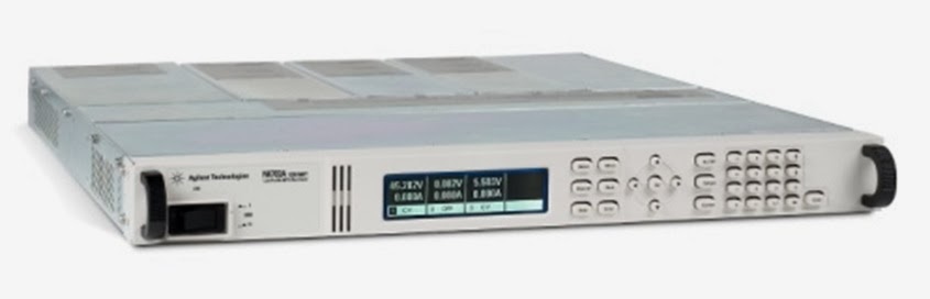
Interestingly this very set up can be programmatically configured within our N6900A and N7900A series Advanced Power System (APS) power supplies. These products have Amp-hour and Watt-hour measurement integrated into their measurement systems. Not only can you measure these parameters, there is a programmable way to act on them in a variety of ways as well, which is the expression signal routing. 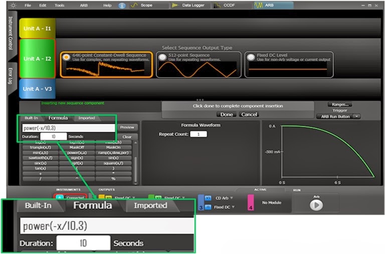Logical expressions can be programmed and downloaded into APS, which then acts on them at hardware-level speeds.  Creating and loading the signal routing expression into the APS unit is simplified by using the N7906A Power Assistance software, which let me do it graphically, as shown in Figure 2.

Figure 2: Graphically developing and loading an energy limit setting into an Agilent APS unit

In Figure 2 a threshold comparator was set to generate a trigger output at a level of 0.0047 watt-hours. This trigger was then routed to the output transient system, to cause the output to transition to a new output level when triggered. I had entered in zero volts as the triggered output level. Thus when the watt-hour reading reached its trigger point, the output went to zero, cutting off any more power and energy from being delivered to the DUT.

The SCPI command set for this signal routing expression is also generated from this software utility by clicking on “SCPI to clipboard”. This saves on the effort generating the code manually if you are incorporating the expression into a larger test program. For this expression the code generated is:

:SENSe:THReshold1:FUNCtion WHOur

:SENSe:THReshold1:WHOur 0.0047

:SENSe:THReshold1:OPERation GT

:SYSTem:SIGNal:DEFine EXPRession1,"Thr1"

:TRIGger:TRANsient:SOURce EXPRession1

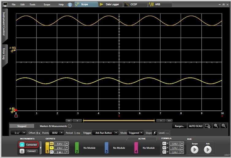
To test things out a 1.18 ohm resistive load was used to draw 84.75 watts for a 10 volt output setting. The output cut back to zero volts at nearly 200 milliseconds, as expected. This is shown in the oscilloscope capture in Figure 3.

Figure 3: APS output for an 84.75 watt load and energy limit set to 0.0047 watt-hours

The load power was then doubled by increasing the output voltage to 14.142 volts. The APS output cut back to zero volts in half the time, delivering the same amount of energy, as expected. This is depicted in the oscilloscope capture in Figure 4.

Figure 4: APS output for a 169.5 watt load and energy limit set to 0.0047 watt-hours

While using a resistor makes it easy to see that a set amount of energy is being delivered to the load. However, being able to act on a real time watt-hour energy measurement makes it very practical to do deliver a fixed amount of energy, regardless of the dynamic nature of the load over time.

Using Binary Data Transfers to Improve Your Test Throughput

From time to time I have shared here on “Watt’s Up?” a number of different ways the system DC power supply in your test set up impacts your test time, and recommendations on how to make significant improvements in the test throughput. Many of these previous posts are based on the first five of ten hints I’ve put together in a compendium entitled “10 Hints on Improving Throughput with your Power Supply” (click here for hints 1-5).

Oscilloscopes, data acquisition, and a variety of other test equipment are often used to capture and digitize waveforms and store large arrays of data during test, the data is then downloaded to a PC. These data arrays can be quite large, from thousands to millions of measurements. For long-term data logging the data files can be many gigabytes in size. These data files can take considerable time to transfer over an instrument bus, greatly impacting your test time.

Advanced system power supplies incorporating digitizing measurement systems to capture waveform measurements like inrush current are no different. This includes a number of system DC and AC power products we provide. Even though you usually have the choice of transferring data in ASCII format, one thing we recommend is instead transfer data in binary format. Binary data transmission requires fewer bytes reducing transfer time by a factor of two or more.

Further details about using binary mode data transfers can be found in hint 7 of another, earlier compendium we did, entitled “10 hints for using your power supply to decrease test time” (click here to access). Between these two compendiums of hints for improving your test throughput I expect you should be able find a few different ideas that will benefit your particular test situation!

Keysight Technologies – What’s in a name, anyway?

This is an exciting time for us! Yesterday, January 7, 2014, we learned what our new company name will be: Keysight Technologies. Here is a link to the official press release: 

http://www.agilent.com/about/newsroom/presrel/2014/07jan-gp14001.html

If you have not heard by now, back in September of 2013, Agilent Technologies announced it would split into two companies by the end of 2014. Since I started in 1980, 33+ years ago, I have worked for and will continue to work for the electronic measurement side of the business. For my first 19 years with the company, we were Hewlett-Packard, a company that formed in 1939 as a test and measurement company and eventually birthed Silicon Valley. It is this electronic measurement side of the business that is getting the new name, just as we did in 1999 when we became Agilent from Hewlett-Packard. The other part of Agilent, the life sciences, diagnostics, and applied markets side will continue to operate under the Agilent name. Note that the electronic measurement side will still have the same great people designing and supporting the same great products and services….just a new name: Keysight Technologies.

So let’s take a closer look at the new name, logo, and tagline for Agilent’s electronic measurement business:

The name combines the words “key”, meaning essential, and “insight” meaning intuitive perception. Essential intuitive perception. Seeing what others cannot. A key can also be used to unlock something; we will continue to unlock measurement insights, as our tagline says. And we have been doing this for 75 years - since the day that Bill Hewlett and Dave Packard released their first electronic test instrument, an audio oscillator, in 1939. By the way, it is purely a coincidence that the Watt’s Up? authors, Ed, Matt, and I have combined experience of more than 75 years as stated in our blog header, although I’d like to think that the three of us have been unlocking measurement insights in the AC and DC power field for a combined total of 75 years! In fact, we now have a total of more than 80 years’ experience between the three of us and I will update the header later this year when we officially begin using the Keysight name. But I digress...

The logo symbol is derived from one of the most fundamental wave shapes there is: a sine wave – a wave shape from which all other wave shapes can be built. This is very appropriate for our 100% focus on electronic measurement, not to mention a tribute to our original founders, Bill and Dave, for their audio oscillator. And the power products and topics that you read about here in Watt’s Up? are equally represented by the logo symbol, especially our AC sources! If you really think about it, Keysight will be doing what Hewlett-Packard originally set out to do and Agilent continued to do for decades: build the world’s leading test and measurement company.

So what’s in a name? Essential intuitive perception is in our name. A clear focus on electronic measurement is in our name. Our strong and deep heritage is in our name. And when we begin to fully operate as Keysight Technologies later this year, what you will find behind our name will be the same high quality products and people that you have come to know. That’s what’s in the name Keysight Technologies!